Interpreting Language Model Parameters

Neural networks use millions to trillions of parameters to learn how to solve tasks that no other machines can solve. What structure do these parameters learn? And how do they compute intelligent behavior?

Mechanistic interpretability aims to uncover how neural networks use their parameters to implement their impressive neural algorithms. Although previous work has uncovered substantial structure in the intermediate representations that networks use, little progress has been made to understand how the parameters and nonlinearities of networks perform computations on those representations.

In this work, we present a method that brings us closer to this understanding by decomposing a language model's parameters into subcomponents that each implement only a small part of the model's learned algorithm, while simultaneously requiring only a small fraction of those subcomponents to account for the network's behavior on any input.

The method, adVersarial Parameter Decomposition (VPD), optimizes for decompositions of neural network parameters into simple subcomponents that preserve the network's input-output behavior even when many subcomponents are ablated, including under ablations that are adversarially selected to destroy behavior. This encourages learning subcomponents that provide short, mechanistically faithful descriptions of the network's behavior that should aggregate appropriately into more global descriptions of the network's learned algorithm.

We study how sequences of interactions between these parameter subcomponents produce the network's output on particular inputs, enabling a new kind of 'circuit' analysis. While more work remains to be done to deepen our understanding of how neural networks use their parameters to compute their behavior, our work suggests an approach to identify a small set of simple, mechanistically faithful subcomponents on which further mechanistic analysis can be based.

1  Introduction

Mechanistic interpretability aims to reverse engineer neural networks, such as language models, so that we can understand the neural algorithms they have learned. Reverse engineering requires decomposing a system into simpler parts that we can study in relative isolation. Unfortunately, it is not obvious how best to decompose neural networks into such parts [1, 2]. The most straightforward candidates for these parts, such as neurons, attention heads, or whole layers, don't always map to individual, interpretable computations [3, 4, 5, 6, 7, 8, 9, 10].

Alternative approaches to decomposition, such as transcoders [11, 12] or mixtures of linear transforms [13, 14], typically involve fitting a set of simple functions to the transitions between activations at different layers in the network, and linearly combining the outputs of these simple functions. The idea here is to approximate the complex, nonlinear function implemented by the network's layers using a simpler, easier-to-understand function. These methods, sometimes called activation-based decomposition methods, have led to significant advances in our understanding of the intermediate representations inside neural networks when computing their outputs [11, 12].

Unfortunately, because the simpler functions that these methods use are of a different functional form to the original network, it is hard to relate their accounts of network function to the actual objects that are doing the computations, namely the network's parameters and nonlinearities.

This is not just a theoretical issue. It prevents us from achieving practical engineering goals. For example, it makes it challenging to know how to make precise, predictable modifications to a model's neural algorithm by making edits to its parameters. It also makes it hard to predict how the model's neural algorithm will perform on a different distribution to the one it was studied on.

The mismatch of functional form between models and their activation-based decompositions is an important issue, but it is not the only one: Activation-based methods have not yet yielded decompositions that exhibit a fully satisfactory level of mechanistic faithfulness [12], and suffer from a number of other issues (See [2] for review).

These issues motivate alternative approaches to mechanistic decomposition, including parameter decomposition methods [15, 16, 17], which give accounts of network function in terms of the parameters that the network uses on each datapoint. Ablation-based parameter decomposition methods [15, 16] aim to identify a set of parameter components where as few components as possible are necessary to perform the same computations as the original network on any datapoint, and "unnecessary" components can be ablated on a given datapoint in any combination without adversely affecting output reconstruction error. Simultaneously, the parameter components are selected to implement as simple computations as possible and to sum collectively to the target network's parameters. If parameter components exhibit all these properties, then they are strong candidates for the network's 'ground truth' mechanisms^[1].

Parameter decomposition methods can identify known ground truth mechanisms in toy models that: Are not necessarily aligned to architectural components such as neurons, individual attention heads, or layers; operate on representations in superposition; or are multidimensional. And, due to the requirement that unnecessary components can be ablated in any combination rather than just all simultaneously, parameter decomposition methods should not exhibit feature splitting. Notably, parameter decomposition methods can readily be applied to any architecture, unlike activation-based methods, where it has been challenging to use the same decomposition methods to decompose both attention layers and MLPs [18, 12, 19, 20]. In demonstration of this ability, previous work has used ablation-based parameter decomposition to identify induction heads in a transformer trained on a toy model of induction [21].

Ablation-based parameter decomposition methods thus promise solutions to many of the issues of activation-based decomposition methods. However, prior parameter decomposition proposals have several important shortcomings, some of which we address in this work with a new method that we introduce, called adVersarial Parameter Decomposition (VPD)^[2]. Our main contributions are:

• We scale parameter decomposition to full language models: While the most recent parameter decomposition method, Stochastic Parameter Decomposition (SPD)[16] is more scalable than its predecessor, Attribution-based Parameter Decomposition [15], it has not yet been applied to full language models. We use VPD to decompose a small language model ($67$M parameters, four layers) trained on the Pile [22]. We find parameter subcomponents that are highly interpretable (Section 3.4), both in terms of the dataset examples that they activate on and how they interact with other subcomponents to produce specific behaviors (Section 5).

• We introduce a stronger notion of ablatability to achieve more mechanistic faithfulness: While some work has applied SPD to a single layer of GPT2-small [21], no application of SPD so far has measured key metrics that would be necessary to ensure mechanistic faithfulness, such as having good output reconstruction loss even under adversarially chosen ablations (rather than under only stochastically chosen ablations). We resolve this issue with VPD, which builds heavily on the SPD method but has several important modifications, which together make it more mechanistically faithful and scalable to larger models than those decomposed in previous work. The primary difference between VPD and SPD is in the ablations. On each datapoint, both SPD and VPD sample from the space of possible partial ablations of parameter subcomponents in order to check whether those parameter subcomponents can be partially ablated in any combination, thus identifying whether they are "necessary" for that datapoint. However, where SPD samples from the space of partial ablations using stochastic samples from the space, VPD uses adversarially chosen samples (Section 2.4) ^[3]. The core details of the method are discussed in Section 2.
• We compare VPD to other decomposition methods: We compare the parameter subcomponents that we find to the objects found by other decomposition methods, such as per-layer and cross-layer transcoder (CLT) latents. We find that VPD achieves a better tradeoff between sparsity and reconstruction under standard training objectives and is more robust to mismatches between training and evaluation protocols compared to end-to-end trained methods (Section 3.3, Appendix B.1). VPD also has comparable interpretability (Section 3.4) and exhibits less feature splitting (Section 3.5) than activation-based comparisons.
• We decompose attention layers into computations that are distributed across multiple heads: Our approach decomposes parameters in attention layers into functionally specialized subcomponents that span multiple heads. These subcomponents interact to perform interpretable computations. Perhaps for the first time, our approach yields a satisfying decomposition of computations in attention layers even though those computations may involve multiple heads (Section 4).
• We develop attribution graphs to study information flow between parameter subcomponents: We demonstrate that the parameter subcomponents found by VPD can be used to construct interpretable attribution graphs that let us study the circuits that underlie some language model behaviors (Section 5).
• We use parameter subcomponents to manually edit a model: Finally, we provide a proof of concept showing that we can use our understanding of the network’s parameters to manually edit a model in a predictable, interpretable way. In particular, we rewrite the part of its neural algorithm involved in emoticon predictions (Section 6).

Additionally, we also introduce an approach for clustering parameter subcomponents into full parameter components. Previous methods left this clustering step implicit [16] (Appendix A.8). We introduce an explicit clustering method, but found that subcomponents were usually interpretable even without clustering, and therefore used clustering only rarely in our analyses.

We release a library for reproducing our experiments and running VPD at https://github.com/goodfire-ai/param-decomp.

2  The core method: adVersarial Parameter Decomposition

In this section, we introduce ablation-based parameter decomposition methods from scratch and highlight key differences between VPD and prior methods in this class. Although our method, VPD, builds heavily on SPD [16], the following explanation of VPD does not assume familiarity with SPD or its predecessor [15].

Our goal is to decompose a neural network into the mechanisms that it uses to compute its behavior. Its mechanisms are what it uses to take input activations, compute its hidden activations, and finally compute its output. We don't approach this goal with strong presuppositions of what a "mechanism" is. But we take for granted that a typical network doesn't use all of its mechanisms on every input (or, at least, it doesn't use all of its mechanisms by the same amount). If that were not the case, then networks could not be said to be modular, having distinct parts that do different things on different inputs. Without modularity, networks simply couldn't be decomposed into separable functional units.

One candidate for the network's mechanisms is the network's parameters. Like mechanisms, networks appear not to use all of their parameters simultaneously on every datapoint [23, 24, 25]. This happens, for instance, when a network's parameters "read from" activation subspaces that are orthogonal to the activations on that datapoint, thus projecting the activations to zero, thereafter having no downstream causal effect. Alternatively, if the activations fail to "activate" a given ReLU neuron, the activation of that neuron is zero, thereafter having no downstream causal effect. However, the network's parameters are in fact a single vector in the network's parameter space, and do not have an obvious decomposition into parts. How should they be decomposed into parts that comprise the network's mechanisms?

On a high level, parameter decomposition methods use the idea that it should be possible, for a given datapoint, to identify the "subset" of the network's parameters that are necessary and sufficient for computing its output on that datapoint. That "subset" of parameters should contain all the mechanisms used by the network on that datapoint. If particular "subsets" of the network's parameters are repeatedly used together by different datapoints, then they may be part of the same mechanism. Parameter decomposition methods therefore aim to find particular "subsets" of the network's parameters that tend to be used together, where as few of them as possible are necessary and sufficient for computing the network's output on any input^[4].^[5]

More concretely: If particular parameters are unused by the network on a particular datapoint, then we should be able to ablate them (including partially) on that datapoint without adversely affecting the network's output. Ablation-based parameter decomposition methods thus aim to decompose network parameters into a set of vectors in parameter space called parameter components. Parameter components are trained to exhibit a number of specific properties such that, if they exhibit those properties, they would be good candidates for the network's "mechanisms". They are trained to be:

• Parameter-faithful: They sum to the network's total parameter vector;
• Minimal: As few components as possible are causally important for computing the network's output on any particular input;
• Mechanistically faithful: Every subset of components that includes the causally important components is sufficient to compute the network's output on any particular input;
• Simple: Each component should involve as little computational machinery as possible.

In the following sections, we define parameter components concretely and explain how they are optimized to exhibit each of these four properties.

2.1  Parameter components consist of subcomponents

Suppose we have a neural network $f(x;\theta)$ with parameters $\theta$. We would like to decompose this parameter vector into a sum of parameter components with the above properties.

It would be computationally expensive to decompose models into whole parameter vectors, since each such vector would have a memory cost equivalent to the whole target model. Therefore, as in [16], we use a less expensive way to parameterize parameter components: Although its parameters $\theta$ can be expressed as a single large vector, they are more commonly conceptualized as a set of matrices $\theta = \{W_1, \dots, W_L\}$. We further decompose individual matrices into sums of rank-one matrices called subcomponents, each parameterized as an outer product of two vectors:

where there may be more subcomponents than rows and columns in the matrix. Permitting more subcomponents than rows and columns in the matrix allows VPD to identify mechanisms that operate on representations in superposition[26, 27, 28].

Although a single subcomponent explicitly parameterizes only a single weight matrix, it implicitly parametrizes a full parameter vector if we assume it takes values of $0$ in all other weight matrices. It is therefore possible to combine these subcomponents into full parameter components by adding them together in the right way. We identify these components using a subcomponent clustering method. Previous work left this clustering step implicit, but in this paper we introduce an explicit method (Appendix A.8).

2.2  Enforcing parameter faithfulness with $\Delta$-components

To ensure the components collectively sum to the parameter vector of the target model, we define additional $\Delta$-components, $\Delta^l$, that parametrize the difference between our subcomponents and the original model's matrices:

We also encourage the $\Delta^l$-components to be small with an auxiliary MSE loss ($\mathcal{L}_{\text{Delta-L2}}$) (Appendix Section A.1).

2.3  Optimizing for minimality

We want as few subcomponents as possible to be causally important for computing the network's output on any particular input. We therefore need some way to estimate which parameter subcomponents are "necessary" for computing the network's output on a given datapoint. We also require a notion of how well the "necessary" subcomponents have reconstructed the network's output.

Ablation-based parameter decomposition methods contend that a parameter subcomponent is "necessary" if it cannot be ablated without affecting the model's output on that datapoint. As in [16], we train a causal importance function to predict how ablatable each subcomponent is on each batch and sequence position. We also implement the causal importance function using a neural network, though we use a different architecture (Appendix Section A.2).

We call the output of this function the causal importance values, $g^l_{b,t,c}\in[0,1]$ (for each subcomponent $c$ of weight matrix $l$ at a given batch index $b$ and sequence position $t$):

• If $g^l_{b,t,c} = 0$, then we should be able to fully or partially ablate that subcomponent on the forward pass at position $b,t$ without affecting the final model output.

• If $g^l_{b,t,c} = 1$, then it should not be possible to ablate that subcomponent without affecting the model's output on that datapoint^[6].

We want as few subcomponents as possible to be required to compute the output, so we train the causal importance values $g^l_{b,t,c}$ to take minimal values with an importance minimality loss:

where $p>0$.^[7]

2.4  Optimizing for mechanistic faithfulness

Components and their causal importances should be mechanistically faithful to the original model. One way of operationalizing this is to insist that, on any given data point, it should ideally be possible to ablate all causally unimportant components from the model weights, using any combination of ablations, without changing the model output. Another, more succinct, way of saying this is that every subset of components that includes the causally important components should be sufficient to compute the network's output on any particular input.

This is a much stricter requirement than merely demanding that the output should be invariant to the joint ablation of all causally unimportant components together. To see why it is stricter, suppose that two components $\theta_A$ and $\theta_B$ can be jointly ablated, but not individually ablated, on a data point without affecting the output^[8]. Then we would consider both $\theta_A$ and $\theta_B$ to be causally important on that datapoint, whereas the less strict criterion might consider them both causally unimportant because they happen to be jointly ablatable. In other words, the stricter criterion demands an unchanged model output over a whole set of points in parameter space, whereas the less strict one demands it only for a single point. For an illustration of why this stricter condition is necessary, see Section 7.3.

VPD works on the level of rank-1 subcomponents instead of full components, but the same principle applies.^[9] To check whether subcomponents are ablatable, we define ablation masks $m^l_{b,t,c}\in[g^l_{b,t,c},1]$ for each subcomponent at each batch index $b$ and sequence position $t$. So, if a subcomponent has causal importance $g^l_{b,t,c}=1$, the only permitted value for the mask $m^l_{b,t,c}$ is also $1$, whereas if the causal importance is $0$, its mask can take any value between $0$ and $1$. These masks define new weight matrices $W^{\prime l}_{b,t}$ which we should be able to insert in place of the original model matrices $W^l$ without substantially changing the model's final output.

We operationalize this by demanding that the KL-divergence $D$ between the model output on the original forward pass and on forward passes using the masked weights should be small:

Ideally, we would calculate this masked reconstruction loss for every permitted combination of ablation masks $m$ for all subcomponents^[10] in all the model's weight matrices, but this would require performing an intractably large number of forward passes. So we instead use ablation masks $m$ drawn using two types of sampling:

1. Stochastic sampling, with ablation masks $m^{\text{stoch}}$ drawn from uniform distributions. This yields the stochastic reconstruction loss, $\mathcal{L}_{\text{stochastic-recon}}$.
2. Adversarial sampling, using ablation masks $m^{\text{adv}}$ optimized via gradient ascent to maximise the reconstruction loss. This yields the adversarial reconstruction loss, $\mathcal{L}_{\text{adversarial-recon}}$.

For details on the stochastic and adversarial sampling, see Appendix Section A.3.

2.5  Optimizing for simplicity

Each component ought to contain as little computational machinery as possible. Otherwise, we could say that the target model is one big parameter component, and proclaim our decomposition complete without doing any actual decomposition!

We both constrain and train our subcomponents to be simple. Our subcomponents are rank-one, which constrains them to be simpler objects than full matrices. Unfortunately, this is not enough of a simplicity constraint, because some rank-one solutions can be "simpler" than others: In some situations, it is possible to add multiple subcomponents parametrizing independent mechanisms used on disjoint subsets of the data together and have the resulting sum also be rank-one.^{[11] [12]}

We therefore encourage breaking up subcomponents into multiple that are causally important on as few data points as possible by introducing an additional, slightly superlinear, penalty on subcomponent activation frequency:

There are probably multiple ways to optimize for the computational simplicity of parameter subcomponents, and we are not confident this choice is optimal (nor our choices for the other losses). Nonetheless, we found it to work well enough in practice. See Appendix Section A.4 for a more detailed motivation of this loss.

2.6  Summary of loss terms

In total, our loss function has five terms:

They each optimize the parameter subcomponents to exhibit particular properties:

• The $\mathcal{L}_{\text{adversarial-recon}}$ and $\mathcal{L}_{\text{stochastic-recon}}$ losses optimize for mechanistic faithfulness (Equation 3).
• The $\mathcal{L}_{\text{importance-minimality}}$ loss optimizes for minimality (Equation 2).
• The $\mathcal{L}_{\text{frequency-minimality}}$ loss optimizes subcomponents for simplicity. They are also constrained to be rank-1 matrices, which imposes one aspect of simplicity (Equation 4).
• The $\mathcal{L}_{\text{Delta-L2}}$ auxiliary loss optimizes for parameter-faithfulness, even without the $\Delta$-components, which ensure it (Equation 1).

The key difference between VPD and our previous work [16] is the $\mathcal{L}_{\text{adversarial-recon}}$ and $\mathcal{L}_{\text{frequency-minimality}}$ losses. There are several other, smaller differences that do not fundamentally change the method but that we found helpful for decomposing language models. For more details, see Appendix Section A.

We evaluate the quality of our decomposition on a number of key metrics. For assessing the quality of a decomposition, the most important are $\mathcal{L}_{\text{adversarial-recon}}$ and $L_0$ per datapoint. For readers looking for practical advice on how to tune hyperparameters and key optimization metrics, we provide a detailed Training recipe for VPD in Appendix A.6.

3  Analyzing language model parameter subcomponents

3.1  Target language model

We trained a four-layer 67M parameter decoder-only transformer model on an uncopyrighted subset of The Pile [22]. A summary of the model architecture and training results can be found in Table 1 and full training details of our target model can be found in Appendix A.7.

Attributes of our target model
Layers	4
Residual stream dimension	768
MLP intermediate dimension	3072
Attention heads	6
Attention head dimension	128
Context length	512
Vocabulary size	50,277
Positional encoding	RoPE [30]
Normalization	RMSNorm [31]
Activation function	GELU [32]
Attention type	Standard Multi-Head Attention [33]
Tied embeddings	Yes
Non-embedding parameters	~28M
Total parameters (incl. embedding)	~67M
Training dataset	The Pile [22] (subset)

We decomposed the 24 weight matrices in this model into a total of of 38,912 rank $1$ subcomponents. We omitted the embedding and unembedding matrices. The decomposition used much fewer than its full capacity, having only ~10,000 alive components (with a mean causal importance greater than $10^{-6}$).

On average, each datapoint uses 205 subcomponents per sequence position, representing 2.1% of all alive subcomponents. Table 2 shows per-layer summary statistics for the decomposition.

Layer	$C$	Alive	Mean L0	L0/Alive
Layer 0	$9728$	$3709$	$44.6$	$0.012$
Layer 1	$9728$	$848$	$18.9$	$0.022$
Layer 2	$9728$	$1943$	$49.5$	$0.025$
Layer 3	$9728$	$3472$	$92.0$	$0.026$
Total	$38912$	$9972$	$205.0$	$0.021$

3.2  The decomposition model behaves similarly to the target model

If a decomposition method has correctly identified the mechanisms underlying a model's computation, then activating only the mechanisms that the method identifies as causally important on a given input should approximately reproduce the model's behavior on that input. Conversely, if a replacement model fails to reproduce the model's behavior, then the decomposition has either missed important mechanisms or identified spurious ones. Reconstruction quality is therefore a necessary (though not sufficient) condition for a decomposition to be mechanistically faithful.

Our parameter subcomponents capture different amounts of the target model's performance depending on how masks are calculated (Table 3). One quantitative measure of performance is cross-entropy (CE) loss on the validation set: The decomposed model achieves between 2.72 and 3.02, depending on the type of sampling, compared with 2.71 for the target model.

A metric that is sometimes helpful for comparison is Pretraining Compute Recovered[34], which is the percentage of the target model's total pretraining compute at which the target model's training curve reaches the same validation CE loss as the reconstruction model (i.e. a value of X% means the reconstruction performs no better than the target model did when only X% of pretraining was complete).

When we exclude the $\Delta$-component (which is trained to be as causally unimportant as possible), the remaining unmasked parameter subcomponents recover about $82\%$ of the pretraining compute. When using stochastic ablations, this drops to around $27\%.$

Masking mode (excluding $\Delta$-components)	Validation CE Loss	Pretraining Compute Recovered (%)
Target Model	2.71	100%
Unmasked (All masks$=$1)	2.72	82.4%
Stochastic Masks	2.84	26.9%
Rounded Masks (Mask$=$1 if CI$>$0)	2.94	11.8%
Rounded Masks (Mask$=$1 if CI$>$0.1)	2.95	11.3%
Causal Importance values (CIs) used as Masks	2.99	9.4%
Rounded Masks (Mask$=$1 if CI$>$0.5)	3.02	8.0%

Pretraining compute recovered is rarely reported, so comparisons to other methods are difficult. Nonetheless, VPD compares favorably to the only other method in the literature that we are aware of that reports this metric: Top-$k$ SAEs [34] reports a pretraining compute recovered of $10\%$ when replacing a single layer of GPT-4 with an SAE with 16 million latents. By comparison, even though our approach decomposes the whole model rather than just a single layer, it recovers between $8\%$ and $27\%$, depending on the ablation method used^[13].

The table below shows KL-divergence to the target model under adversarial masking with different numbers of adversarial optimization steps, calculated across a batch of $128$ of sequence length $512$ drawn from the evaluation set ^[14].

Adversarial optimization steps $n^{\text{adv}}$	KL divergence to target model
20	0.8280
40	1.3539
80	3.8381
160	25.2560
320	40.2200

While the decomposition is somewhat robust to approximately $20$ steps of adversarial optimization, it is clearly not at all robust to $160$ steps or more.^[15]

However, we note that complete adversarial robustness would not necessarily be desirable. See Section 7.3 for some discussion of how much adversarial robustness a decomposition ought to exhibit to be considered mechanistically faithful.

Qualitatively, the generations produced by different sampling methods align with the above quantitative measures. The generations seem qualitatively to produce similar behavior to the target model in most cases (Figure 3).

Surprisingly, even when masks are adversarially sampled with 20 steps of adversarial optimization, the generations are not entirely nonsensical. This is feasible because we only get to adversarially sample causally unimportant parameter subcomponents.

3.3  VPD has a better tradeoff between reconstruction versus sparsity compared with transcoders

Any decomposition of a neural network faces a fundamental tradeoff between the number of `objects' they use to reconstruct the network's behavior and the quality of that reconstruction. If a decomposition can use fewer objects to capture the same amount of network performance, then that explanation is preferred according to Occam's razor, assuming the objects use a similar amount of computational machinery.

We study the reconstruction versus sparsity tradeoffs of different decompositions and compare the VPD model with two families of activation-based decomposition methods: Per-layer transcoders (PLTs) [11] and cross-layer transcoders (CLTs) [10], both using BatchTopK [36]. We simultaneously replace all 4 MLP layers of the target model with their sparse reconstructions and measure the resulting increase in cross-entropy loss relative to the unmodified target model.

There isn't a straightforward apples-to-apples comparison between transcoder latents and VPD subcomponents, so we present a number of different comparisons (with more extensive experimental details in Appendix B.1) ^[16]. To ensure our conclusions are not artifacts of how we count subcomponents or latents, we show results under three possible definitions of sparsity:

1. Average active subcomponents per module: Active encoder latents for PLTs/CLTs; active subcomponents per weight matrix for VPD;
2. Active subcomponents per MLP Down reconstruction: Adjusting for the fact that a CLT latent affects multiple layers and that VPD uses two modules per MLP;
3. Total active parameters: VPD's rank-one subcomponents have more parameters than a PLT latent and a single CLT latent has multiple decoder vectors.

We compare VPD with PLTs and CLTs trained with their standard training losses, noting these are different objectives (VPD trains on output reconstruction while PLTs and CLTs are trained to reconstruct activations at each layer).

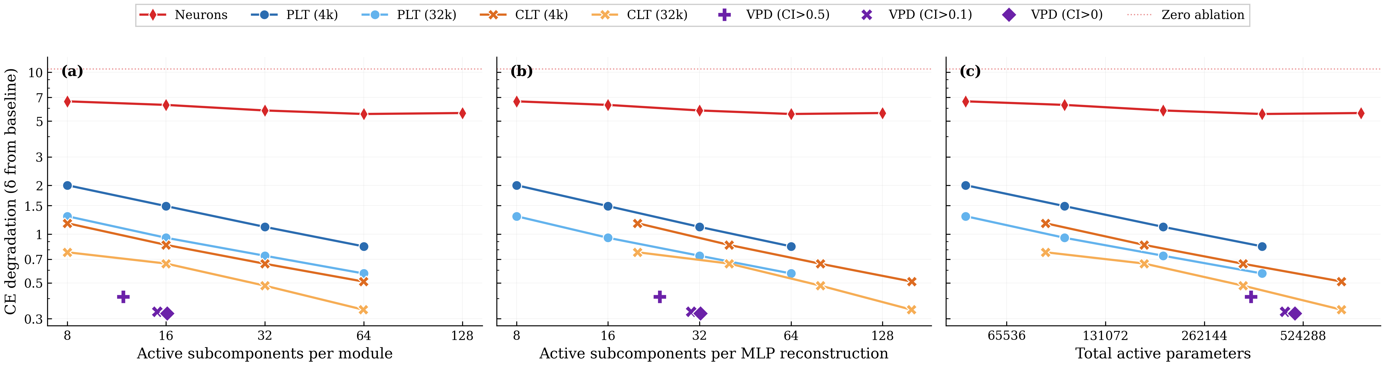
We observe that VPD performs favorably compared with activation-based decomposition, achieving less CE degradation for a given $L_0$ across all three definitions of sparsity.

We noted above that VPD and the transcoders differ in training objective. VPD is trained end-to-end, whereas activation-based approaches are usually trained layerwise. This complicates direct comparison and arguably makes the above analysis somewhat unfair to activation-based methods. We address this by also comparing under matched objectives in Appendix B.1 and find that VPD compares favorably to other methods: When trained and evaluated on a range of objectives, VPD's Pareto domination disappears, but it avoids overfitting to its particular training objective, unlike the activation-based methods.

Additional figures and training logs for the VPD decomposition can be found at the WandB link here.

3.4  Parameter subcomponents are highly interpretable

In order to study a parameter subcomponent's role in the network's neural algorithm, we need a definition of what it means for it to be 'active' on a given datapoint.

There are at least two reasonable definitions:

1. Causal importance: The causal importance function is trained to output a value between $0$ and $1$ that tells us exactly how important a particular subcomponent is on a datapoint. It tells us if the subcomponent is 'necessary' or 'required' or 'used' on that input. In many ways, this is a perfect definition of 'active'! However, it is not a 'local' measure of a subcomponent's activation: A subcomponent with a small causal importance value might interact strongly with the activations at a layer, only for its effect to be suppressed later by others. For a more 'local' measure, we use the next definition.
2. Subcomponent activation: We define the subcomponent activation as $$a_c^l = ||\vec{U}^l_c|| (\vec{V}^l_c)^\top \vec{\varphi}^l,$$ where $\vec{\varphi}^l$ are the model's hidden activations before matrix $l$ ^[17]. This defines how much the activations interact with a given subcomponent, even if that interaction ultimately ends up not being causally important for the output. Due to superposition [37, 38, 28, 26, 27], there will be more interactions in general than there are causally important interactions.

Throughout this paper, we use both definitions, highlighting which type of activation we mean in each instance.

We find that parameter subcomponents tend to 'activate' (in both senses) for coherent categories of inputs. Figure 5 shows some dataset examples on which each subcomponent is causally important. It also shows the subcomponent activation in the underlines. You can navigate the panel to explore the activations of a variety of parameter subcomponents:

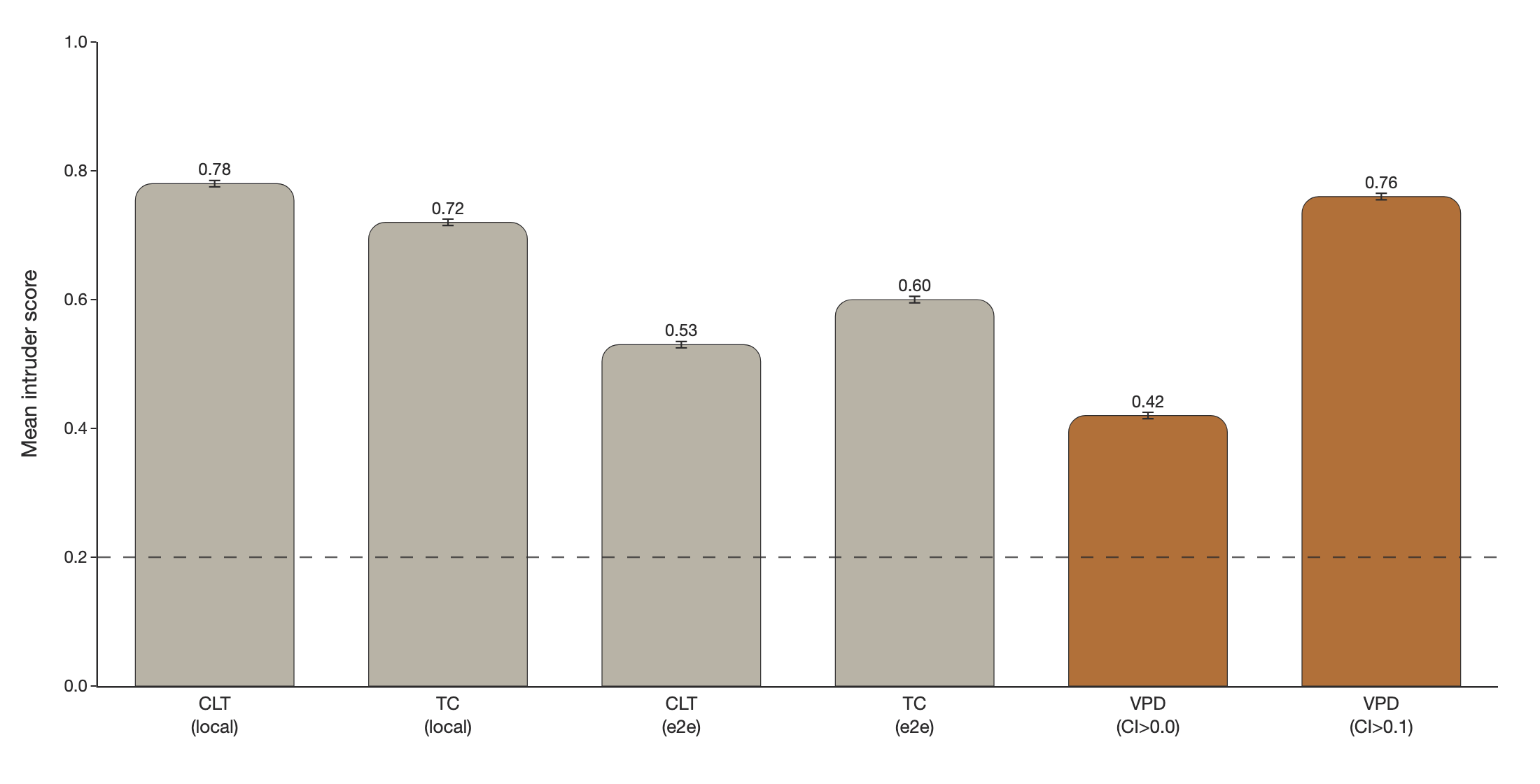
To compare how 'interpretable' parameter subcomponents are relative to transcoder latents, we can measure how semantically coherent a subcomponent's activation patterns are using intruder detection [39, 40]. In intruder detection, we present an LLM-judge with a set of inputs that activate a given VPD subcomponent or transcoder latent alongside one 'intruder' example that does not activate it. We task the LLM-judge to identify the intruder example. It should be easier to identify the intruder among a more semantically coherent set of inputs. In the VPD setting, we use causal importance values in place of activation magnitudes and select intruder examples with similar activation densities.

We find VPD intruder detection scores improve drastically when using CI values thresholded with 0.1, which filters low-CI noise Figure 6. We think that filtering out small causal importances is justifiable, since 0.1-rounded performance has essentially the same performance as 0.0-rounded performance, suggesting that very little performance is captured by subcomponents with small activations (Table 3).

We observe that 0.1-rounded VPD subcomponents score competitively with CLTs and PLTs trained using a local (layerwise) MSE activation reconstruction loss Figure 6. VPD subcomponents are more coherent than PLTs and CLTs that were trained end-to-end.

3.5  VPD does not suffer from feature splitting

Feature splitting is a well-known issue in activation-based dictionary learning methods such as PLTs, SAEs, and CLTs [41, 42]. As dictionary size increases, these methods can improve sparsity and reconstruction by replacing a 'broad', reusable latent with several narrower, more context-specific ones. In the extreme, a transcoder could assign a unique latent to every individual datapoint in the training set, effectively memorizing the dataset rather than uncovering reusable, general patterns.

VPD does not suffer from this issue, either in principle or in practice. The key reason for this is that subcomponents marked as causally unimportant are required to be ablatable in any combination, not just all simultaneously. The model therefore needs to be robust to variations in parameter space along the directions of these subcomponents for all batches and sequence positions, not just the ones on which they are causally important. Without this constraint, the decomposition might be able to invent overly 'narrow', context-specific subcomponents that do not actually exist in the computational structure of the original model but that sparsely activate while reconstructing the model's behavior on some narrow subset of the data. For example, suppose VPD attempted to pathologically decrease $\mathcal{L}_{\text{importance-minimality}}$ by splitting a mechanism in the target model that ought to be parametrised by two subcomponents into many specialised subcomponents that lie within that mechanisms' two-dimensional subspace, each aligned with a different training-data hidden activation vector, and marked only one of them at a time as causally important. If we were just using the causal importances as masks, this would reconstruct the target model's output well. But with stochastic or adversarial masking, many of the subcomponents not marked as causally important will be turned on as well, making the resulting output activation vector both too large and pointed in the wrong direction, thus ruining the reconstruction. See Section 7.3 for further discussion.

To test empirically whether VPD does avoid feature splitting, we incrementally increase the number of subcomponents used by different VPD runs and count the number of "alive" subcomponents (subcomponents that activate at least once every 1M tokens). We train VPD at four capacity levels corresponding to $0.5\times$, $1\times$, $2\times$, $4\times$ the subcomponent count of the main decomposition we study. We compare against PLTs and CLTs at 4k and 32k dictionary sizes.

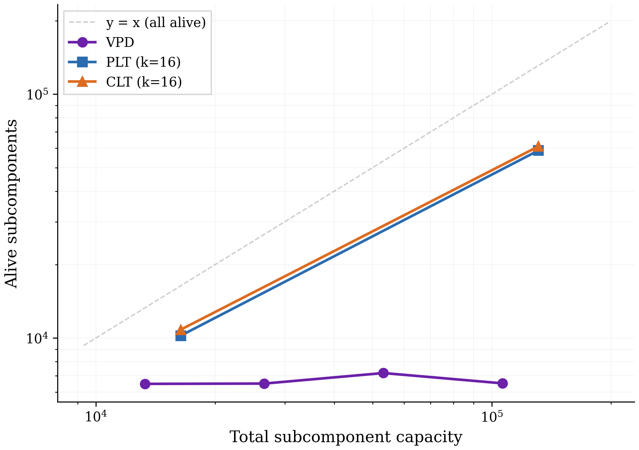
Figure 7 shows that, unlike PLTs and CLTs, increasing VPD's capacity does not increase the number of subcomponents that the method actually uses, suggesting that feature splitting is not a significant problem for VPD. Across all four VPD runs the sparsity and reconstruction performance remain approximately constant, so the flat alive count reflects unused capacity rather than a tradeoff against sparsity or reconstruction. In Appendix B.2, we confirm that our PLTs and CLTs are indeed splitting features rather than discovering genuinely new ones.

While we only show results for one language model here, we have observed the same qualitative result in every model we have decomposed with either VPD or SPD [16] despite extensive hyperparameter sweeps, including various toy models with known ground truth and a smaller language model trained on the SimpleStories ([43]) dataset.

4  Decomposing attention behaviors that are distributed across attention heads

Transformer language models are significant in large part because they were the first architecture that enabled scalable sequence modelling. The crucial component that lets transformers perform computations across sequences is the attention layer ([33, 44]).

In most prior work that studies attention layer computations, attention heads have typically been the primary units of analysis to study attention behaviors [45, 46, 47, 48, 49, 7, 50]. Unfortunately for interpretability, it is possible for attention layers to perform computations in a way that is distributed across multiple heads [8, 51]^[18]. It would therefore be ideal if our decomposition methods could cope with attention computations that are distributed across heads. So far, it has been difficult to find satisfactory activation-based decomposition methods that can do this [51, 52, 53, 54, 18].

Fortunately, parameter decomposition methods offer some hope: As we've seen in Section 3.4, parameter subcomponents seem to decompose the parameters into specialized functional units. And since parameter subcomponents are vectors in parameter space, they can therefore span multiple attention heads!

In this section, we demonstrate that parameter subcomponents in attention layers are indeed interpretable, and can span multiple attention heads (and usually do!). Focusing primarily on attention layer 1, we study three attention layer behaviors ('Previous token behavior', 'Previous syntactic boundary movement', and 'Detecting Existential vs. Expletive Constructions') and show how parameter subcomponents distribute these computations across heads.

4.1  Attention layer parameter subcomponents have specific interpretable roles

First, we look at a few parameter subcomponents in attention layer 1. In this layer VPD identifies different numbers of parameter subcomponents in the $W_Q$, $W_K$, $W_V$, and $W_O$ matrices. These matrices have 15, 48, 226, and 97 alive^[19] components respectively, though we'll usually present fewer for simplicity.

There are many interesting subcomponents in these matrices that correspond to easily interpretable behaviors:

• L1.Attn.q:308 activates on tokens related to existence or the verb 'to be' and other 'copula' verbs.
• L1.Attn.k:485 activates on words that predict 'copula' verbs, such as ·there or ·it in "there is/it is".
• L1.Attn.k:218 activates on the word ·it (including capitalized variations and variants both with and without a leading space)
• L1.Attn.k:119 activates on punctuation, spaces, brackets, newlines and other 'interstitial' words.
• L1.Attn.k:290 activates on newlines and end-of-text tokens only.
• L1.Attn.v:42 activates on coordinating conjunctions, like ·and, ·or, ·but and ·&.
• L1.Attn.v:178 activates on words related to position in time and, to a lesser extent, space, like ·December, ·South, ·2002, ·long and ·far.
• L1.Attn.o:983 Activates on the introductions or titles of texts, particularly scientific papers.

Additionally, there are some subcomponents whose role seems more related to 'sequence position' than having a particular semantic meaning:

• L1.Attn.q:149 and L1.Attn.q:497 tend to activate on the tokens immediately following the first token of the sequence (and, incidentally, reveal some of the shortcomings of our autointerp labelling method, which seems to have missed this!).
• L1.Attn.k:315, L1.Attn.k:357 and L1.Attn.k:121 tend only to be causally important on the first few tokens of a sequence, though with some exceptions.

Together, these interpretations are encouraging, because they suggest that our decomposition is identifying parts of the network that are specialized for particular functional roles.

4.2  Attention layer parameter subcomponents typically span multiple heads

We've seen evidence that attention subcomponents are specialized for specific semantic roles, suggesting different computational functions. Now we investigate whether these subcomponents are 'located' in particular heads.

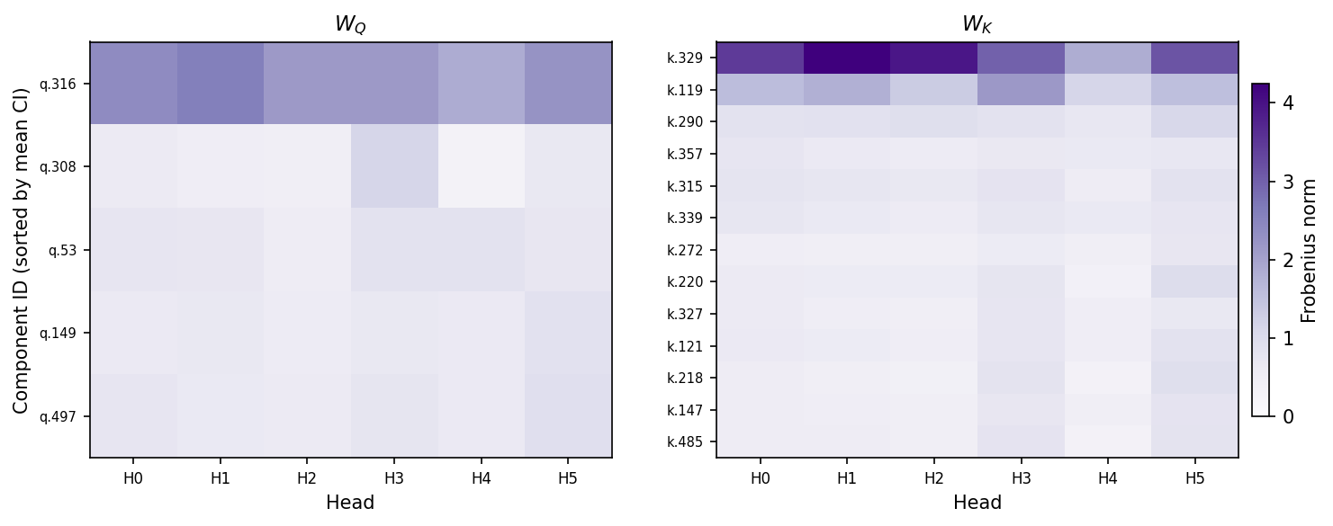
In our model, the $W_Q$, $W_K$, $W_V$, and $W_O$ matrices are concatenated across attention heads. But we can easily split them into the matrices belonging to individual heads. Even though parameter subcomponents by default span all heads in a layer, most of their 'mass' could be localized in single heads if their weights in all but one attention heads have zero norm. But if their parameters have nonzero norm in multiple heads, then this is weak evidence that they perform computations across multiple heads.

We'll focus on the $W_Q$ and $W_K$ matrices for now. We see that, in fact, most $W_Q$ and $W_K$ subcomponents have nonzero weight norm across each head (Figure 8). This suggests that most $W_Q$ and $W_K$ subcomponents might perform computations in a distributed way! The norms subcomponents of $W_V$ and $W_O$ matrices seem similarly distributed across heads (Figure 28)

While suggestive, this is only indirect evidence of distributed computations. We would need to understand the computations in order to confirm that they are indeed distributed across heads. To do this, we will need new analysis tools. And we can make the problem slightly easier by separately studying the two main parts of the attention layer: The QK circuit and the OV circuit [47]. We'll focus on the QK circuit first.

4.3  The QK circuit consists of interactions between pairs of parameter subcomponents

In attention layers, $W_Q\in \mathbb{R}^{d_{\text{model}}\times d_{\text{model}}}$ and $W_K\in \mathbb{R}^{d_{\text{model}}\times d_{\text{model}}}$ matrices transform sequences of activations $\varphi\in \mathbb{R}^{T\times d_{\text{model}} }$ in the (normed) residual stream to create queries ($q = \varphi (W_Q)^\top $) and keys ($k = \varphi (W_K)^\top$) for all heads. We can split them into the keys and queries for each head (e.g. $q = [ \varphi (W_Q^{1})^\top, \cdots , \varphi (W_Q^{H})^\top]$).

The attention scores of head $h$ are calculated as $Z^h = \varphi W_Q^{h \top} W_K^h \varphi^\top$, which are used to calculate the head's attention pattern, $A^h = \text{softmax} (Z^h) $.

Although the $W_Q$ and $W_K$ matrices are usually represented as separate matrices, it is convenient to study them together as a single matrix, $W_{QK}^h = W_Q^{h \top} W_K^h$ [47].

Prior to parameter decomposition, it was not obvious how best to further decompose this circuit into specialized functional units. But VPD decomposes the $W_Q$ and $W_K$ matrices in a sum of functionally specialized rank-one parameter subcomponents ^[20]:

These subcomponents are secretly also a decomposition of the QK circuit, constructed from pairs of subcomponents of the $W_Q$ and $W_K$ matrices:

(5) $$ \begin{aligned} W_{QK}^h &= W_Q^{h \top} W_K^h \\ &= \left( \sum_c \vec{U}^{h}_{Q,c} (\vec{V}_{Q,c})^\top \right)^\top \left( \sum_{c'} \vec{U}_{K,c'}^{h} (\vec{V}_{K,c'})^\top \right) \\ &= \sum_{c, c'} \vec{V}_{Q,c} \left( (\vec{U}_{Q,c}^{h})^\top \vec{U}_{K,c'}^h \right) (\vec{V}_{K,c'})^{\top} \end{aligned} $$

We will use this equation to study the QK circuit, both for a form of static (data-independent) and dynamic (data-dependent) analysis of the computations of the QK circuit.

We'll need to define two new metrics, one to measure the static interaction strength between pairs of subcomponents and another to measure how strongly a pair of subcomponents are interacting on a particular datapoint.

QK Circuit - Metric 1: Static Interaction strength

Although we can use Equation 5 to understand the static interaction strength between subcomponents $c$ and $c'$, we cannot simply use the raw term $\left( (\vec{U}_{Q,c}^{h})^\top \vec{U}_{K,c'}^h \right)$ for a few reasons:

First, because both $\vec{U}_c$ and $\vec{V}_c$ vectors are unnormalized, we need to scale each $\vec{U}_c$ vector by the norm of the corresponding $\vec{V}_c$ vector in order to put the $\vec{U}_c$ vectors on the same scale.

Second, we need to incorporate sequence position information. The above equations actually leave out an important part of our transformer language model: The Rotary Position Embedding (RoPE) rotation matrix [30]. For transformers that use RoPE, the QK circuit is actually: $W_{QK, \tau}^h = (W_Q^{h})^\top \boldsymbol{R}_{\tau} W_K^h$, where $\tau$ is the offset—the difference between the sequence position of the query and the key. The rotation matrix rotates the keys and queries by different amounts depending on the offset. Thus we have

Third, and finally, we need to know whether this interaction typically contributes positively or negatively to the attention score. To calculate this, we cheat slightly and import one data-dependent statistic: The sign of the average subcomponent activation for each subcomponent on tokens where the subcomponent is causally important. With these three adjustments, we get the Static Interaction Strength:

The Static Interaction Strength metric is not directly comparable across heads, since each head applies a separate softmax function, making any differences in scales or averages of interaction strength irrelevant. To make the metric comparable across heads, we standardize it:

where $\mu_h$ and $\sigma_h$ are the mean and standard deviation of the Static Interaction Strengths across all $(c, c', \tau)$ for head $h$.

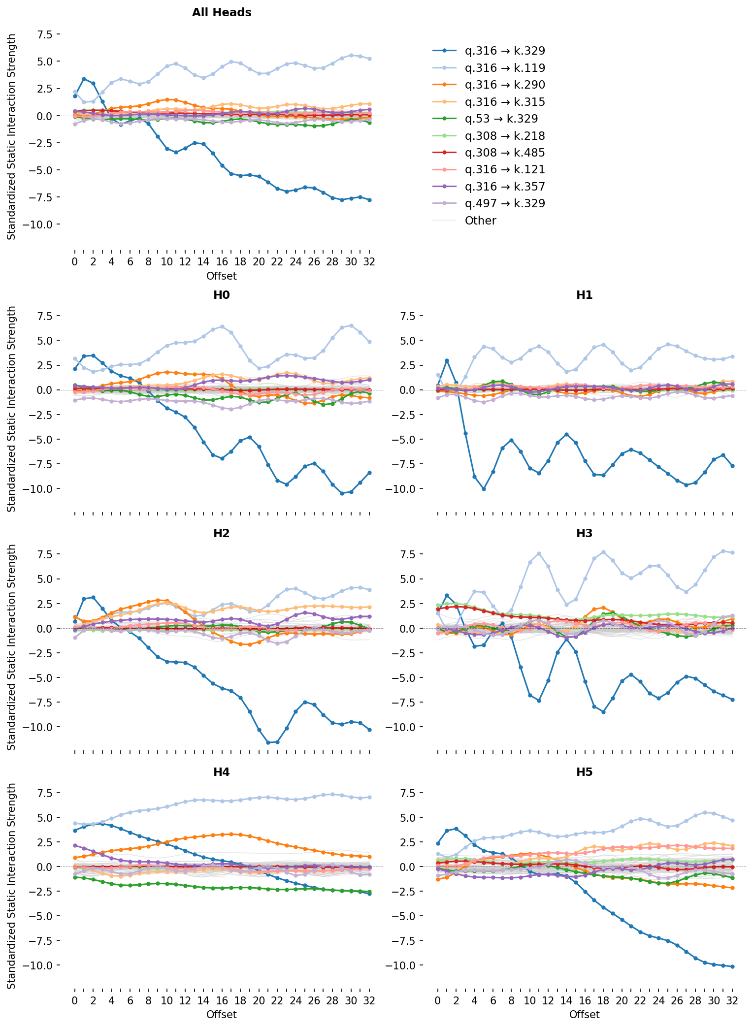
For attention layer 1, we plot this metric for each pair of subcomponents for each head and offset (Figure 9). We can see that for some pairs, the Static Interaction Strength changes strongly at different offsets. This means that, for these pairs, the same activations might have different effects on the attention at different offsets! For others, the Static Interaction Strengths seem independent of offset, meaning that their effects on the attention scores are determined only by whether data that activate them are present.

We will use this plot of Static Interaction Strength to analyze particular attention behaviors. But before we do, we will equip ourselves with a related metric, the Data-Dependent Interaction Strength, which permits dynamic analysis.

QK Circuit - Metric 2: Data-Dependent Interaction Strength

The attention patterns of each head depend on how the hidden activations interact with the QK circuit: $A^h_\tau = \text{softmax} (\varphi W_{QK, \tau}^{h} \varphi^\top)$.

We can use Equation 5 to decompose the QK circuit and study how the activations $\varphi$ at different timesteps $t,t'$ interact with each of the pairs of subcomponents:

Thus, the attention score at each head $h$ and offset $\tau$ consists of the sum of the data's interaction with each of the individual pairs $(c, c')$. On any input, we can therefore decompose the attention score—and hence the attention pattern—into parts that we can study in isolation. This lets us define a data-dependent metric of interaction strength, which forms the basis of our dynamic analysis:

If we broadcast this over sequence position and head, we can visualise a subcomponent pair's interactions across a whole prompt as a stack of per-head matrices — and the model's full attention score $Z$ as the (per-head, per-position) sum of every such pair. To keep the figure readable, we'll abbreviate the position-independent pair term as

In Figure 10, you can select which subcomponent interactions to sum together and see the attention score for those pairs. This is a very useful tool, since it splits up any given attention pattern into the contributions of individual, functionally distinct, subcomponent interactions.

We'll do an initial analysis of an attention behavior using only these two QK metrics before discussing how they interact with the OV circuit.

4.4  Decomposing attention behavior 1: Previous token behavior

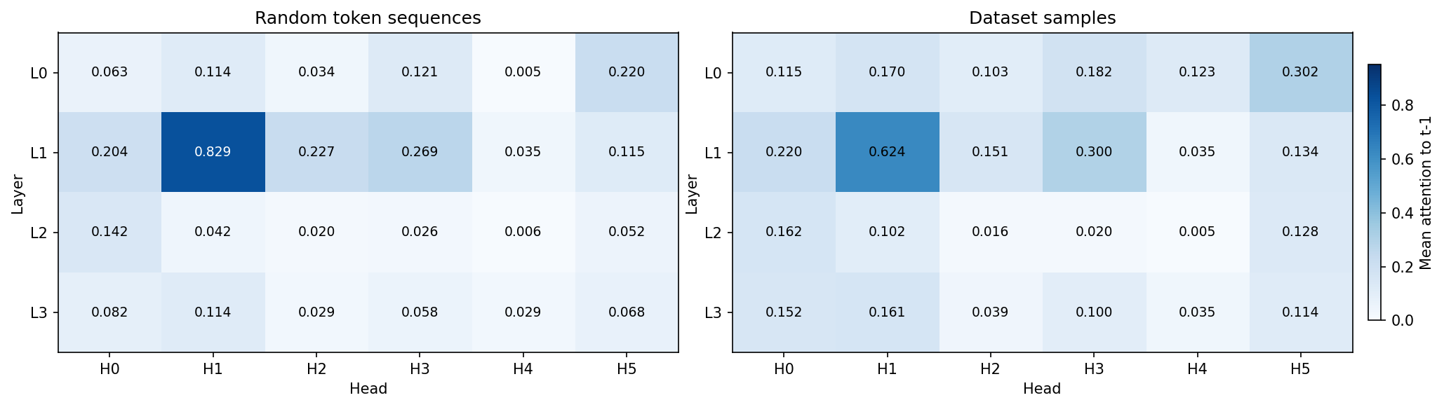
Like many language models, our model has a head that, on average, places the majority of its attention on the previous timestep (Figure 11). This is typically called a previous token head [55, 47, 48, 49] and, in our model, is head 1 in layer 1 (L1H1). However, L1H1 is not the only head to assign substantial probability to the previous token; many other heads do too, including heads in the same layer as L1H1.

Now we need to find subcomponents that might be involved in previous token behavior and establish whether or not their computations span multiple heads. An obvious place to start is by looking at the largest, most frequently active subcomponents in the $W_Q$ and $W_K$ matrices. Perhaps by coincidence, the largest norm subcomponents, L1.Attn.q:316 and L1.Attn.k:329, are also the most frequently causally important (Figure 8)!

While most subcomponents in layer one are only active on a fraction of tokens, both L1.Attn.q:316 and L1.Attn.k:329 have a CI firing density of $96.7\%$ and $99.8\%$, meaning they're nearly constantly active. Both have the largest weight norm in L1H1, which was the head with the strongest previous token behavior (Figure 8). But they also have substantial weight norm in other heads, suggesting they aren't exclusively located in any particular head. Could they be responsible for cross-head previous token behavior?

Figure 9 shows that these two subcomponents also have very strong offset-dependent Static Interaction Strength. In particular, their interaction is strongest at small offsets, and weak or negative interactions at more distant offsets. This is exactly what we would expect of two subcomponents that implement previous token behavior or recent token behavior. This pattern holds not only in L1H1, but also in other heads too. This is strong observational evidence that these two subcomponents compute previous token behavior in a way that is distributed across heads.

We test this hypothesis causally using ablations and dynamic analysis. When we ablate different $W_Q$ subcomponents on a dataset of prompts, the change in average attention is very small for most subcomponent ablations. Only the ablation of L1.Attn.q:316 results in the large reduction of attention at recent offsets (Figure 12).

Figure 10 shows dynamic analysis. For any of the prompts, you can remove the contribution of the L1.Attn.q:316 and L1.Attn.k:329 interaction to the attention score. Removing it destroys the attention to tokens in the recent past across all heads that had strong to moderate attention there.

Together, this is strong evidence that the L1.Attn.q:316 and L1.Attn.k:329 interaction computes previous token behavior and is distributed across heads.

This raises a question: What information is this attention moving from the recent past to the current timestep? What attention values does this previous token behavior tend to move? Are the different heads carrying forward information from distinct subspaces in the residual stream? Or are they carrying redundant information, perhaps as a form of noise robustness? To study this, we need to analyze the OV circuit, for which we will need another metric.

Previous token behavior employs non-overlapping subspaces in the OV circuit

The OV circuit is made from the $W_V$ and $W_O$ matrices which respectively read from and write to the residual stream:

The sequence of $T$ vectors of dimension $d_{\text{model}}$ that the attention layer outputs into the residual stream is computed using the attention pattern-weighted sum of the outputs of the OV circuits at all previous timesteps (where the attention pattern $A^{h}$ is determined by the QK circuit):

Although $W_{OV}^h$ is a $d_{\text{model}} \times d_{\text{model}}$ matrix, it only has rank $d_{\text{head}}$. Being low rank, each head can therefore only read from and write to a small subspace of the residual stream. It would be useful to know if two heads read from and write to similar subspaces.

To do this, we will measure the 'overlap' between the subspaces that each head's OV circuit reads from and writes to, for which we'll use the 'Data-weighted Subspace Similarity' metric, which we construct from the Frobenius cosine similarity of the 'read subspaces' and the 'write subspaces' of each head (Figure 13). See Appendix B.6 for details of how these subspaces are constructed and for further details of this metric. We also measure the Frobenius cosine similarity of the $W_{OV}^h$ matrices themselves (Figure 13). When calculating similarity, we weight the axes of the read- and write-subspaces by how much data variation lies in each axis, since we do not care as much about weight similarity along axes where data do not exist or do not vary. In all cases, we compare the measured similarities to similarities between random, data-weighted matrices.

Most heads in layer 1, except L1H4, seem at least weakly involved with previous token behavior, as assessed by their previous token score (Figure 11) and the offset dependence of the Static Interaction Strength of the L1.Attn.q:316 and L1.Attn.k:329 pair (Figure 9). We therefore should look at the overlap in the read and write subspaces of all heads in layer 1 except L1H4.

The read subspaces of each head are close to or slightly lower than the expected similarity of two random (data-weighted) matrices (Figure 13). On the other hand, the write subspaces seem close to or slightly higher than the random baseline. These effects seem very weak, but weakly suggest a pattern of attention heads reading from distinct subspaces but writing to slightly less distinct subspaces.

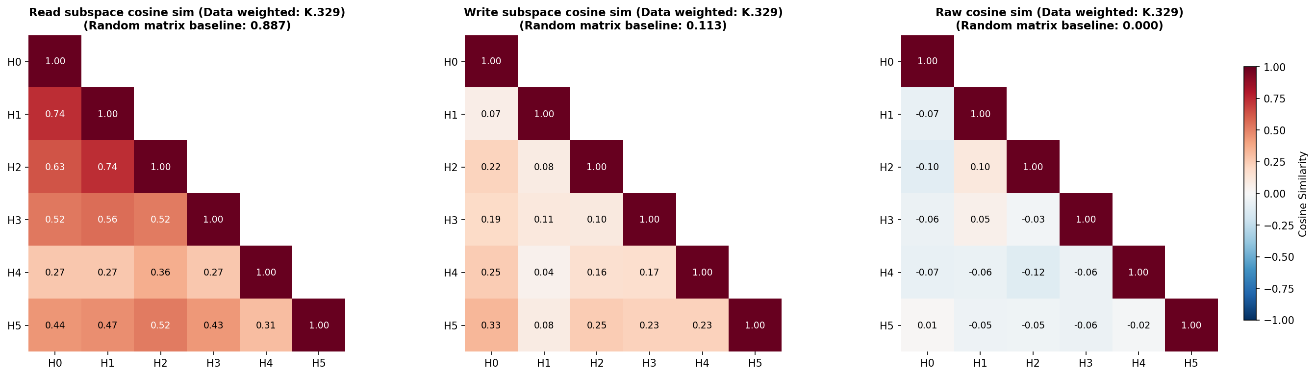
For the head with the strongest previous token behavior, L1H1, the other heads L1H0 and L1H2 seem to read from subspaces with similarities close to the random baseline, but other heads read from much less similar subspaces. When comparing the similarity of the raw $W_{OV}^h$ matrices, there appears to be very little deviation from levels of overlap that would be expected of random matrices, except the comparison between L1H1 and L1H2, which again seem to be more similar than the random baseline. These two heads seem to write to quite different subspaces, though.

Overall, this weakly suggests a picture that previous token behavior spans distinct subspaces across different heads. One potential reason for this is to be able to read more information from the residual stream than might be readable by a single head. There appears to be very limited, but nonzero, redundancy in how heads involved in previous token behavior read from different subspaces, but they largely seem to write to different subspaces.

Previous token behavior is an important behavior implemented by probably every language model. But it is far from the only behavior implemented in layer 1. Even in L1H1, only around 60% of attention is on the previous timestep (Figure 11). What other attention behaviors is this head implementing? In the next section, we look at another behavior implemented by L1H1 in more detail, and examine whether that behavior is also distributed across heads.

4.5  Decomposing attention behavior 2: Previous syntax boundary movement

Looking again at the static analysis of layer 1, we can see that L1H1 has interactions between Q and K subcomponents that seem to have quite a different offset-dependency (Figure 9). The subcomponents L1.Attn.q:316 and L1.Attn.k:119 seem to interact most strongly at later offsets across multiple heads, including L1H1.

We are already familiar with L1.Attn.q:316, the query subcomponent that is always active. The key subcomponent L1.Attn.k:119 is new: It seems to activate on brackets, punctuation, and newlines, but also some common continuation words, such as 'the' or 'and'. It is causally important on 16% of tokens, which is frequent, but not constantly active.

This interaction therefore involves a conditional computation: Although L1.Attn.q:316 is always active, constantly looking back in time, the other subcomponent L1.Attn.k:119 only interacts with it when it is active.

Interestingly, L1.Attn.k:119 must be active sufficiently far back in time; otherwise, the Static Interaction Strength may not be strong enough to contribute to the attention score. Almost every head seems to exhibit an offset dependent interaction between subcomponents L1.Attn.q:316 and L1.Attn.k:119, suggestive of a very distributed computation.

Since this computation is data-dependent, we will benefit from greater use of dynamic analysis. Figure 14 shows the attention patterns of all heads, but only shows the Data Dependent Interaction Strength of the L1.Attn.k:119-L1.Attn.q:316 interaction. One prompt is shown at a time, but you can select a variety of other prompts from the dataset in the dropdown menu.

By exploring different prompts, and inspecting the contributions of the L1.Attn.q:316 and L1.Attn.k:119 interaction across all heads, it is possible to see that this interaction contributes significantly to the attention patterns of most heads on previous periods, commas, and newline characters. L1H4 seems capable of maintaining attention on these characters at quite large offsets, based on the stronger than average vertical bars in the ground truth attention on those tokens. Other heads seem only to have noticeable attention on them more recently in time. This may be due to competition with other attention score contributions from other pairs.

The activating examples of L1.Attn.k:119 show firings on various forms of punctuation, end of text tokens, newlines, latex "$" symbols, brackets, etc. This suggests that this pair of subcomponents orchestrates a syntax boundary detector with a variety of short- or long-offset ranges. We'll call this 'previous syntax boundary' movement.

This pair of subcomponents seems responsible for attention to syntax boundary tokens at different ranges in different heads (Figure 9). L1H1 seems to increase self attention upon syntax boundary tokens; L1H2 seems only mildly to attend to syntax boundary tokens and only in the very recent past. L1H5 and L1H0 attend to syntax boundary tokens a small number of tokens in the past. L1H4 seems to attend to syntax boundary tokens many tokens in the past. L1H3 is less clear, but seems to attend to a smaller subset of specific syntax boundary tokens, usually with shorter offset ranges.

The QK circuit of the 'previous syntax boundary movement' behavior seems quite distributed across heads. How does it interact with the OV circuit? We can study this by looking at probability of each key subcomponent being active conditioned on a given value subcomponent being active (Figure 29). The value subcomponents most associated with L1.Attn.k:119 are:

• L1.Attn.v:72 - fires on punctuation to predict newlines and connectors
• L1.Attn.v:22 - punctuation, syntax, and formatting tokens
• L1.Attn.v:745 - formatting symbols, operators, and spatial alignment
• L1.Attn.v:919 - fires on newlines and indentation
• L1.Attn.v:531 - opening parentheses, brackets, braces, and quotes
• L1.Attn.v:494 - predicts line breaks or indentation in formatted text
• L1.Attn.v:195 - fires on delimiters and structural punctuation
• L1.Attn.v:612 - fires on closing delimiters (parentheses, braces, brackets, math)
• L1.Attn.v:984 - fires on punctuation and symbols
• L1.Attn.v:1000 - fires on punctuation, delimiters, and structural boundaries
• L1.Attn.v:22 - punctuation, syntax, and formatting tokens
• L1.Attn.v:389 - delimiters and punctuation in structured text and code
• L1.Attn.v:188 - structural punctuation and syntax symbols
• L1.Attn.v:299 - fires on commas and semicolons
• L1.Attn.v:1014 - subordinating conjunctions and relative pronouns
• L1.Attn.v:227 - fires on periods and member access operators
• L1.Attn.v:946 - distinguishes content words from function words/symbols
• L1.Attn.v:340 - syntactic linkages and prepositions
• And some with weaker associations (Figure 29).

As in the case of previous token behavior, the data-weighted OV circuits (where we weight the similarity using dataset examples and tokens where L1.Attn.k:119 is causally important) do not seem to read from very similar residual stream subspaces (Figure 30), though they seem to write to somewhat more similar subspaces than would be expected in random matrices. The OV circuit subcomponents that subcomponent L1.Attn.k:119 seems to overlap strongest with are associated with other punctuation and syntax boundary-like tokens across seemingly all heads, in both the read and the write matrices (Appendix B.9).

To understand why the model is carrying forward information about the previous syntax boundary, we would need to know how the values are being used downstream. But it is possible to surmise at least part of its function: It is useful to know what the previous syntax boundary tokens are in order to perform tasks like closing opened brackets; knowing whether a list is a bullet list or dashed list; or knowing if a token is within or outside of a quotation; and more.

4.6  Decomposing attention behavior 3: Detecting Existential vs. Expletive Constructions

Both of the above attention behaviors (Section 4.4 and Section 4.5) have involved $W_Q$ or $W_K$ subcomponents where one is 'always active'. Although the vast majority of the attention scores in this layer seem to involve at least one of these subcomponents, it would be interesting to study an even more conditional behavior.

We'll investigate an attention behavior involving the $W_Q$ subcomponent L1.Attn.q:308 - fires on existence and state verbs (is, was, there are/is).

This subcomponent appears to activate on a subset of copula verbs. Examples of copula verbs include:

• "To be" ("she is", "it was", "What were", ),
• Verbs related to sensory appearance ("it certainly seems", "she appeared as though", "they looked like"), and
• Verbs related to state ("we remain", "it becomes readily apparent", "there exists").

Grammatically, copula verbs behave as linking verbs: They connect a subject ("it", "she", "there", "we", etc.) to a description or complement, rather than expressing an action. They are relatively ubiquitous throughout English, so it makes sense that even a small language model would learn computations involving them.

Subcomponent L1.Attn.q:308 activates on a subset of copula verbs

Although L1.Attn.q:308 has a large subcomponent activation on copula verb tokens, it is noteworthy that it is not causally important on all instances them. Here are several prompts containing copula verb tokens on which L1.Attn.q:308 is not causally important on some tokens despite having high subcomponent activation:

By contrast, here are a few prompts where L1.Attn.q:308 is causally important on copula verb tokens:

By studying the difference between these two sets, it is possible to notice a pattern: Although L1.Attn.q:308 has a large positive subcomponent activation on most instances of copula verbs, the cases where it is causally important are typically when it is preceded by it, there, here (as in "it is", "there is", "there are", "here is", "makes it seem") and related tokens.

Constructions like these have specific linguistic terms: Existential and expletive constructions, which use "there" and "it" in particular senses:

• The 'existential "there"': Where "there" is used to make assertions about the existence of something. Examples: "There is a problem", "there wasn't enough", "there seems to be several", "there exists", "there have been few attempts", "there remains a number of"

• The 'expletive "it"': Where "it" is used as a dummy subject, with no real referent. Examples: "It is unusual", "It appears likely", "It was found that", "It dawned on him that"^[21], "It looks like"

Even though L1.Attn.q:308 has a high subcomponent activation on most copula verbs, it is usually not causally important (with some exceptions) when the copula verb is preceded by personal pronouns (e.g. "she", "he", "they"):

How could this be? The main way that QK subcomponents can influence downstream computations (and hence have causal importance) is by influencing attention. L1.Attn.q:308 having a large subcomponent activation is insufficient for attention. There needs to be a key subcomponent that aligns with L1.Attn.q:308 (i.e. has a high Static Interaction Strength) that also has a high subcomponent activation in order for a Q-K subcomponent pair to have high Data Dependent Interaction Strength, and hence to contribute significantly to the attention pattern. There must therefore be $W_K$ subcomponents that L1.Attn.q:308 'looks for' in the past that, if present, give this subcomponent its causal importance.

Subcomponent L1.Attn.q:308 interacts with two specific $W_K$ subcomponents

We'll start looking for this interaction by looking at whether there are subcomponents that have a high Static Interaction Strength with L1.Attn.q:308.

Looking again at Figure 9, we can see that L1.Attn.q:308 has strongest offset-dependent Static Interaction Strength with two $W_K$ subcomponents, namely L1.Attn.k:218 and L1.Attn.k:485. These two interactions are strongest in L1H3, but also in L1H5.

Incidentally, the norm plot (Figure 8) supports the idea that L1.Attn.q:308 is primarily located in L1H3, and secondarily in L1H5, since the weight norm is largest in those two heads and negligible elsewhere.

These two $W_K$ subcomponents (L1.Attn.k:218 and L1.Attn.k:485) seem to be causally important on related, but semantically distinct, tokens, which we explore in detail in the following sections.

Subcomponents L1.Attn.k:218 and L1.Attn.q:308 make an "it + copula verb" detector

L1.Attn.k:218 - fires on the pronoun 'it' predicting subsequent verbs seems to have high subcomponent activation on any instance of the word "it", including capitalized variants. It is also causally important on any instance of the word "it", but its causal importance tends to be higher on instances of the 'expletive "it"'^[22].

The phrase "it is" is often an 'expletive "it"' followed by a copula. But it may also be an 'anaphoric pronoun "it"' followed by a copula, as in "It is mine". It turns out that L1.Attn.k:218 is causally important on both types of "it is". But it is not causally important for expressions involving other pronouns followed by copulas, such as "he is", "they are", etc. It therefore seems that this pair of subcomponents interact to implement an "it + copula verb" detector, including both 'expletive "it"' and 'anaphoric pronoun "it"' followed by a copula

We can see its Data Dependent Interaction Strengths in the figure below. The interaction strengths are strongest in L1H3, with a small amount in L1H5, with essentially none in any other head. The attention patterns reveal that the L1.Attn.q:308 subcomponent 'looks back in time' from copula verbs, and has high Data-Dependent Interaction Strength with L1.Attn.k:218 if it finds it. If it does, it usually contributes enough to the attention score that it becomes causally important.

It turns out that it is quite an overzealous "it + copula verb" detector. It often produces high Data Dependent Interaction Strength even at quite large offsets, even when the "it" and the copula verb are not related to each other. For an example, see the prompts below where a copula verb late in the prompt attends back to an unrelated it token in an earlier sentence:

The L1.Attn.k:485-L1.Attn.q:308 interaction plays a mostly overlapping role to the L1.Attn.k:218-L1.Attn.q:308 interaction

The other subcomponent with which L1.Attn.q:308 has a strong interaction is L1.Attn.k:485 - predicts existence or copula verbs after "there" / "it". It has strongest subcomponent activation on the word "there", but also activates for "here" and "it" (and all their capitalized variants). It tends to be causally important when any of these words is followed by a copula verb.

Together, this indicates that the interaction between L1.Attn.k:485 and L1.Attn.q:308 causes attention to existential constructions, such as "There is", "Here are", "There exists", as well as expletive constructions (which we studied in detail in the previous subsection). This means that its function overlaps with the function of the L1.Attn.k:218 and L1.Attn.q:308 interaction, which also detects expletive constructions.

However, the L1.Attn.k:485-L1.Attn.q:308 interaction contributes relatively less attention to expletive constructions compared with the interaction between L1.Attn.k:218 and L1.Attn.q:308. For example, in the prompt below, the L1.Attn.k:485-L1.Attn.q:308 interaction misses the 'expletive "it"' in "make it probable" while L1.Attn.k:218-L1.Attn.q:308 detects it and causes attention to it.

These two interactions thus both play overlapping, but somewhat specialized roles in detecting what type of construction a copula verb is in.

Both QK subcomponent interactions have similar OV circuits

Their overlapping, but slightly distinct, roles are reflected by their OV circuits.

If either L1.Attn.k:218 and L1.Attn.k:485 are causally important, the $W_V$ subcomponents with the highest probability of also being causally important are (Figure 29):

• L1.Attn.v:744 - fires on pronouns and determiners

• L1.Attn.v:180 - fires on pronouns and dummy subjects (it, there)

• L1.Attn.v:946 - distinguishes content words from function words/symbols

• L1.Attn.v:649 - fires on <|endoftext|> to predict document start

However, both $W_K$ subcomponents do not have identical relationships with all $W_V$ subcomponents. Subcomponent L1.Attn.v:448 - fires on 'there/where/here' predicting 'to be' verbs seems only to have a high conditional probability of being causally important with L1.Attn.k:485, not L1.Attn.k:218. Combined, these values seem to be carrying both grammatical and 'content' information. It's worthwhile noting that these $W_V$ subcomponents are not localized to particular heads, and therefore their information may be mediated via more than one head (Figure 28).

On a normative level, why does the model learn these two behaviors and implement them in this way? On one level, the answer is somewhat obvious: These constructions (existential, expletive, anaphoric) tend to be followed by different types of text, which therefore demands different kinds of predictions. On another level, it feels likely that a better model could have implemented better detectors. To determine whether layer 1 is simply too early in the model for a 'cleaner' implementation, or whether the model is simply too small, would require further investigation. We leave those investigations, as well as studies of how these overlapping, but separable, detectors influence downstream computations, to future work.

We have barely scratched the surface of the extent and complexity of attention computations of even this small model. Nonetheless, we are excited by the possibilities for understanding attention computations opened up by decomposing attention layer parameters into parameter subcomponents. We believe the breadth of this analysis could be massively increased and note there is significant room for increasing the depth analysis that use parameter subcomponents to decompose and understand attention. We have not, for instance, studied how parameter subcomponents could interact across attention layers, perhaps forming structures akin to 'virtual attention heads', but decomposed into their constituent parameter subcomponents.

5  Interpreting circuits of parameter subcomponents

So far, we have studied parameter subcomponents individually, or one attention layer at a time, looking at how they combine within a single attention layer to produce behaviors like previous-token movement and previous-syntactic-boundary movement. But the outputs of a language model are computed using many layers in series. In this section, we use parameter subcomponents to understand at least some aspects of the target model's internal computations from the input embedding all the way to the output on a few different prompts.

To make sense of these multi-step computations, we need a way to study how information flows between parameter subcomponents throughout the entire model. We do this by calculating attributions, which measure the strength of the interaction between causally important subcomponents on particular prompts. The resulting attribution graphs let us trace, on individual prompts, how information moves between subcomponents across layers. In particular, we use gradient attributions, but use stop-gradients on every node other than the source and target so that we measure only the 'direct' effects of one subcomponent on another (Section 5.1).

It should be noted that using gradients in this way 'abstracts away' the complexity of non-linear interactions between subcomponents by summarizing them into a single number. As a result, such attributions are only 'local' measures of interaction strength; their value depends on the particular datapoint that we measure them on. Many works have pointed out issues (such as saturated softmax functions in attention layers) that can cause such local attributions to be unrepresentative of more 'global' measures [56, 57]. In order to identify more 'global' measures of interaction strength, we would need to better characterize the nonlinear relationships between parameter subcomponents. This is an important research priority, and one that we've already begun exploring, but not something that this paper covers in detail. We do nonetheless provide analysis that suggests parameter subcomponents of MLP matrices, despite not being directly selected to have simple interactions, tend toward it anyway (Appendix B.11).

5.1  Attribution calculations

To calculate attributions between two subcomponents, we leverage gradients. In particular, we calculate the gradients between each "subcomponent activation", $a^l_c = (\vec{V}^l_c)^\top \vec{\varphi}^l$. However, we do not always simply use $\frac{\partial a_{c}}{\partial a_{c'}}$, the partial derivative of the target subcomponent activation $a_{c}$ with respect to the source subcomponent activation. The partial derivative measures the influence of $a_{c'}$ on $a_{c}$ through both direct and indirect pathways. Understanding the direct effects of a subcomponent give us the clearest mechanistic picture of its role in the network's neural algorithm. We therefore need an attribution method that can distinguish between direct and indirect effects, unlike the partial derivative $\frac{\partial a_{c}}{\partial a_{c'}}$. But, complicating matters further, in models with residual streams a subcomponent's direct effects are not limited only to those in the immediate next layer. The direct effects may skip many layers!

Instead of using the partial derivative $\frac{\partial a_{c}}{\partial a_{c'}}$, we use the fact that we can control how gradients flow on the backwards pass. We take the partial derivative $\frac{\partial a_{c}}{\partial a_{c'}}$, but we stop the gradients flowing through all subcomponents that are not the source subcomponent (Figure 15). This avoids measuring their effects on the target node, including the indirect effects of the source node that flow through them.

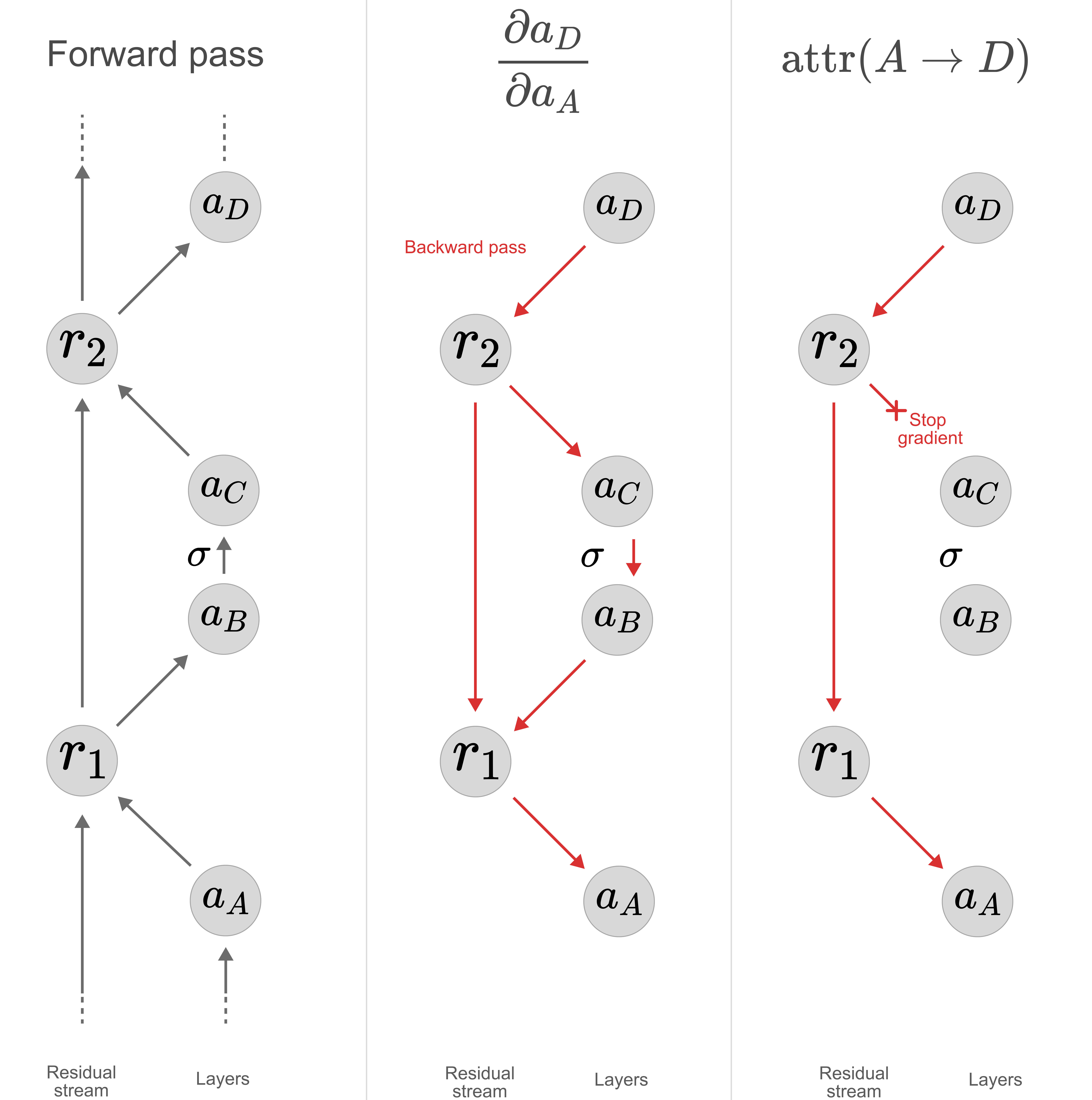
This derivative approximates how sensitive the target node is to the source node. Our attribution multiplies this "sensitivity" by the strength of the activation of the source node in order to measure its overall influence. Additionally, we do not want to include causally unimportant nodes in our attributions, and therefore multiply the resulting term by the source subcomponent's causal importance:

where the $*$ around the partial derivative denotes stopped gradients on non-source subcomponents.

For more details on our gradient attributions, see Appendix B.10.1.

5.2  Pruning for specific behaviors

Most prompts, even simple ones, tend to activate hundreds of parameter subcomponents, which is too many to analyze at once!

We can further reduce the number of subcomponents we need to analyze by keeping only those subcomponents involved in computing some particular output behavior on a prompt that we are interested in.

To do this, we use two types of pruning methods, yielding two types of attribution graph. We'll use both types in our analysis below:

• Attribution graph type 1: Pruning with adversarial sampling: Suppose, on the prompt The ·princess ·lost ·her ·crown ., we wanted to analyze how the model successfully predicts ·her. We would therefore only be interested in subcomponents that were involved in computing this specific prediction at this specific sequence position, which is a smaller subset of subcomponents than the set used to predict all tokens at all sequence positions. We can therefore find new causal importances to identify only those subcomponents by minimizing a set of masks while demanding that cross-entropy reconstruction loss on the label ·her on the sequence position for ·lost remains good. This is different from standard VPD training, which instead used KL-divergence to all the target model's output probabilities on all sequence positions of the prompt. As in VPD training, we optimize causal importances under both stochastic and adversarial mask sampling to try to ensure that the resulting graphs are mechanistically faithful. For details about this technique, see Appendix B.10.2.

One might wonder whether adversarial sampling is actually necessary for mechanistic faithfulness for this post-hoc pruning. After all, the parameter subcomponents are now frozen and only the causal importances can change, so the optimization has much fewer degrees of freedom to create spurious graphs that score well on the loss. To investigate this, we use the second type of attribution graph:

• Attribution graph type 2: Pruning with only causal importances as masks (no stochastic or adversarial sampling): We can also make attributions graphs by making a new set of causal importances. But in this case, we minimizing the causal importances without stochastic or adversarial sampling. We still demand that cross-entropy reconstruction loss on the label ·her on the sequence position for ·lost remains good, but this is much easier because we no longer need to be robust to stochastic or adversarial sampling of the causal importance masks. optimize the graph only for the nodes that are necessary for making a specific prediction (as in the previous type of graph).

In the case studies, we will see that graph type 2 often looks interpretable and contain far fewer subcomponents than the adversarially pruned graphs (type 1). This is somewhat misleading: Because they are not robust to adversarial ablations of parameter subcomponents, type 2 graphs will yield mechanistically unfaithful accounts of the network's computations. They claim that many components are causally unimportant (ablatable), when in fact they are important (unablatable under adversarial sampling), making them look much simpler and more superficial than would a mechanistically faithful account of the the network's computations. Further confirming the mechanistic unfaithfulness of the non-adversarially pruned graphs, they often score much better on the task than the actual target model, reaching near $100\%$ accuracy.^[23] Importantly, we believe that this issue is likely to apply in any setting in which masking-without-adversarial-sampling is used to identify subsets of nodes (or 'subnetworks') in large causal graphs that are important for downstream tasks, which includes a large fraction of the neural network subgraph identification literature to date.

The most important type of graph that we study below is type 1 (Pruning with adversarial sampling), but we will use type 2 to demonstrate the necessity of choosing subcomponents such that the subgraph is robust to adversarial sampling, if our aim is to give mechanistically faithful accounts of the network's computations.

5.3  Case study 1: Gendered possessive pronoun

On the prompt The ·princess ·lost ·her ·crown . the target model correctly predicts with high probability ($0.586$) that ·her follows ·lost. This requires recognizing that a possessive pronoun is likely to come next, remembering that the previous token was ·princess, and knowing that princesses are predominantly associated with female pronouns. How does the model perform this task?

We can use attribution graphs to follow the flow of information between parameter subcomponents and see what information is processed and by which parameters.

The top two pathways in the adversarially pruned graph suggest two core mechanisms: one which moves the femaleness attribute of ·princess over to the next token via attention layer 3, and another which detects the verb ·lost via MLP layer 2 and suggests that an object pronoun might follow.

If we prune the graph for high probability on ·her using only the causal importances as masks, neglecting adversarial robustness, we recover a graph of just six subcomponents (Figure 17), which corresponds almost exactly to the most attributed subcomponents in these same two top pathways.

This confirms that these six subcomponents are sufficient for reproducing the desired output. This much smaller graph even generalises to slightly different prompts: On the input The lady ·lost ·her ·crown ., a forward pass using only the six subcomponents in the small graph at the exact same sequence positions also recovers the target model's ·her prediction^[30]. But the lack of adversarial robustness in the smaller graph confirms that it does not provide anything close to a full account of the relevant computation going into the model's prediction.^[31] All 150 subcomponents in Figure 16 likely play some role — otherwise the optimization would have pruned them. While these six subcomponents suffice to put high probability on ·her, they fail to suppress other computational pathways that would predict different outputs. We do not attempt to fully understand the complete graph here.

How similar are the structures of graphs for slightly different prompts? To investigate this, we run the same analysis on the prompt The ·prince ·lost ·his ·crown ., where the target model predicts ·his with probability $0.512$. We recover similar, but not identical results.

As with the princess prompt, pruning with CI masking instead of adversarial masking recovers a much smaller graph of just six subcomponents organised into two pathways that is sufficient to compute the ·his prediction, but isn't adversarially robust at all.

We stress again that the above is far from a complete account of the meaningful computation going on in the model for these input prompts. We have merely traced out the flow of information between a subset of subcomponents that are sufficient for computing the output, which is much smaller than the subset of subcomponents that are actually involved in computing the output.

5.4  Case study 2: Bracket closing

On the prompt < u , v > the target model correctly predicts that > follows v, assigning probability $0.547$. This requires the model to remember that, earlier in the sentence, < opened a bracket that now needs to be closed. How does the model perform this task?

Notably, in the attention layer 2 of this graph, information about the open bracket seems to be moved from the < position to the v position, partly due to information previously received from the < position in attention layer 1. This triggers a query that is specific to closing-delimiters (such as >), which searches for a preceding opening-delimiter (such as <) key.

Since the $W_Q$ subcomponents used in attention layer 1 and 3 appear to be generically always-active rather than triggering in response to preceding commas, and the queries in layer 2 do not appear to only trigger conditional on a comma at the previous token either, one might wonder whether the model would also predict a closing > right after u. It turns out that it does — predicting > as its top logit after u as well, though with lower confidence ($0.119$ vs. $0.547$ after v). Figure 21 shows a structurally similar graph for this prediction, but lacking the subcomponents active on u and , in the attention layers. This suggests the longer context reinforces the math context and thus the likelihood of a closing bracket. Interestingly, the model does not predict a closing bracket after ,, suggesting it recognises that the comma indicates the statement inside the bracket is not yet complete.

Pruning with CI masking instead of adversarial masking recovers a much smaller graph of just 14 subcomponents (Figure 22). It predicts > correctly under CI masking but fails completely under adversarial masking, giving a very incomplete account of the computation. Nevertheless, it highlights some core pathways.

While the 14-component graph highlights the core pathways, the full graph in Figure 20 makes clear that the actual computation is far more intricate.

Given how few subcomponents our decomposition has in total (ca. 10,000 alive in the whole model) it is perhaps remarkable how many of them appear to be dedicated to moving around and processing information for predicting closing delimiters of various kinds. This may be partially due to delimiter closing being one of perhaps relatively few prediction tasks that is simple enough for a model of this size to perform well.

6  Editing a language model's parameters by hand to modify its neural algorithm

One of the subtasks in language modelling is predicting tokens that comprise emoticons, such as :), :-(, XD, ;), or =).

We used the decomposition to perform a simple edit to the model's learned algorithm: Manually modifying a single rank-1 subcomponent to make the model predict that all emoticons are surprised-face emoticons.

The challenge here is to make models predict the token o, as in a surprised-face emoticon : o, with high probability without substantially altering the model's behavior in other, non-emoticon contexts. Because :/;/X/= (etc.) tokens can be used in many non-emoticon contexts, this rewrite can't be achieved with a token-level remapping; we have to rewrite the algorithm that the model applies to its hidden activations.

We find that multiple subcomponents in the MLP Down matrix of layer 2 specifically activate on the first characters in emoticons with low or zero activations elsewhere, including on these same tokens in other contexts:

• L2.MLP.down:1672 - predicts emoticon continuations after colon or equals
• L2.MLP.down:2359 - punctuation marks starting an emoticon
• L2.MLP.down:2623 - emoticon starter tokens predicting the rest of the emoticon
• L2.MLP.down:3290 - predicts emoticons and smiley faces
• L2.MLP.down:3327 - promotes emoticon completions after colons or semicolons
• L2.MLP.down:3382 - predicts emoticon continuations after colon, semicolon, or equals

We picked one of these subcomponents, L2.MLP.down:2359, as our target for editing. Our edit leverages the idea that each subcomponent, being a rank-1 matrix $\vec{U}^l_c (\vec{V}^l_c)^\top$ has one 'read' direction and one 'write' direction, which are its right and left singular vectors respectively. We changed the 'write' direction of the subcomponent so that, when it activates, it writes very strongly to the same direction as the o token in the model's unembedding matrix.

We performed this edit by replacing the subcomponent's write vector $\vec{U}^l_c$ with $-\alpha\vec{u}_o / \lVert \vec{u}_o \rVert$, where $\vec{u}_o$ is the unembedding direction for the token o^[39]. The new weight matrix thus becomes

To measure the amount of undesired off-target effects caused by the edit, we use two metrics, which characterize off-target effects in slightly different ways, one measuring effects on tokens that are potentially computationally 'nearby' to our edit, and the other measuring all changes:

• $D_{\text{KL},\text{Surrounding}}$: The KL-divergence between the target model and the edited model on the $20$ tokens before and after a token on which L2.MLP.down:2359 is causally important;
• $D_{\text{KL},\text{Global}}$: The KL-divergence between the target model and the edited model on all tokens on which L2.MLP.down:2359 is not causally important, sampled from the whole dataset.

As baselines for comparison, we trained two conventional LoRA adapters for the MLP Down projection matrix in layer 2. The LoRAs were trained to convergence on $n$ dataset examples ($n=10$ or $947$). The training dataset examples consisted of the token on which the subcomponent L2.MLP.down:2359 is causally important and the 20 tokens before and after. They were trained both (a) to predict an o after the emoticon's initial token (e.g. :) and (b) to minimize the off target effects. Concretely, for (a), each LoRA was trained with a cross-entropy loss to predict the o label after the token on which the subcomponent is causally important. For (b), off-target effects were minimized using a KL divergence term (weighted by the off-target effect penalty coefficient, $\lambda$) between the output logits of the target model and the logits of the edited model on the rest of the tokens in the example^[40].

To give a sense of the effectiveness of the VPD edits and the LoRA baseline, Figure 23 shows the per-token KL divergences to the target model for both the VPD edit and the LoRA baseline.

In Figure 24 we vary both $n$ (the number of training dataset examples) and $\lambda$ (the off-target effect penalty coefficient) for our LoRA baselines. We plot the trade-off between the probability of predicting an o versus off target effects. We compare the LoRAs with our manual edit with different scale factors $\alpha$ for the o unembedding vector added to the subcomponents’ $\vec{U}$ vector of L2.MLP.down:2359.

LoRAs trained on just $n=10$ examples outperform the manual edit on $D_{\text{KL},\text{Surrounding}}$, the setting they were trained on, but not on $D_{\text{KL},\text{Global}}$. LoRAs trained with $n=947$ examples outperform the manual edit on both $D_{\text{KL},\text{Surrounding}}$ and $D_{\text{KL},\text{Global}}$.

While this is a promising result, we stress that this is a very preliminary investigation. The method we used to edit the subcomponent, adding the appropriate unembedding vector, was simply the first interpretable editing technique we tried. Other editing techniques might work better. For example, although this edit clearly affects the output in the intended way, there is another layer in between our edited layer and the output, which may lead to some of our edits' off target effects. We may be able to do better by choosing a direction that maximally avoids affecting the computations of the intermediate layer while still projecting strongly onto the o token in the unembedding matrix. This may help to close the gap between the performance of our edit and the performance of the LoRA.

On the other hand, the example is cherry picked. We deliberately chose this task because the model seemed to have a small number of subcomponents related exclusively to emoticon prediction. We nevertheless conclude that VPD shows some promise for model editing in cases where correctly labeled data for training a LoRA is difficult to obtain, or where it is desirable for the edit to be somewhat interpretable. We think that there are very likely ways to leverage parameter decomposition to do much better editing than we have here in this proof of concept.

7  Discussion

At this point, it is worth reflecting on what our parameter decomposition approach has actually bought us with regard to the highest-level goals of our field:

In mechanistic interpretability, we aim to reverse engineer the computational machinery of neural networks. In particular, we want to know how that machinery takes inputs, computes hidden representations, performs computations on those hidden representations, and finally computes its output behavior. Concretely, this means that the objects we want to understand are the computational graphs of neural networks and how they interact with data. To make this as manageable as possible, we'd like to understand small parts of these computational graphs of short description length in isolation, yet have our explanations aggregate together so that, eventually, we can come to understand the entire network as a whole.

In the following sections, we discuss how VPD makes progress toward these goals, or how it does not.

7.1  Parameter decomposition makes fewer assumptions about neural networks' representations than other methods

Parameter decomposition methods are less opinionated than other popular decomposition methods about the 'form' of the computation that we expect to find in neural networks. Sparse dictionary learning methods, such as transcoders or cross-layer transcoders, effectively train replacement models to substitute for parts of the original model, using different architectures with significantly wider layers that are often also composed of different non-linear units. These replacement architectures can have greater representational capacity than the original model, and consequently correspond to entirely different function classes. As a result, they can implement computations that would not be representable using the original model architecture. To ensure these replacement models are mechanistically faithful to the computations in the model, we therefore need to have a somewhat clear idea of the form of those computations ex ante, and use that knowledge to choose the right replacement model architecture and hyperparameters. Otherwise, the replacement models might learn a different internal structure entirely. Feature splitting is one example of this issue.

In contrast, parameter decomposition methods always stay within the confines of the original model architecture. Parameter components are effectively just a different set of coordinates for representing the target model's parameters. Every combination of parameter components corresponds to a valid weight vector we can implement in the original model architecture. In a sense, we're letting the network itself tell us what the form of its computation is instead of guessing a particular form in advance.

7.2  Explanations of attribution graphs are not explanations of computational graphs

A full explanation of a network's behavior should amount to an end-to-end algorithm that is essentially equivalent to the algorithm implemented by the target network. In other words, it should be possible to represent the explanation as a computational graph that is mechanistically faithful to the computational graph of the original network, which is typically expressed in terms of its neurons, weights matrices, nonlinearities, etc.

By contrast, in this paper, we used VPD to produce attribution graphs rather than computational graphs. It is not possible to compute the model output on a datapoint using only the attribution graph without access to the original model itself. An attribution graph can track how strongly any given upstream node in a computational graph influenced any given downstream node, which is useful for understanding the flow of information in the graph, but it does not represent the functional relationship between upstream and downstream nodes. This means we have not yet explained the network's computational graph; the explanations of the model's behavior we provide here are incomplete. Additionally, attribution methods such as the gradient attributions we used in this paper also have some well-known issues that can lead them to misjudge the magnitude of the influence one node in a graph has on another [58, 56]. For example, if an attention head in a model has a saturated softmax, gradient attributions through it will tend to systematically underestimate the effect of ablating the upstream node on the downstream node. Despite these limitations, we think attribution graphs are still useful as a basic picture of how information flows between VPD subcomponents on a forward pass, and have been used to similar effect for other decomposition methods, such as CLTs [12].

In future work we aim to deepen our study of full computational graphs by studying in detail the interactions of VPD subcomponents at nonlinearities, such as MLP neuron activation functions. For some preliminary investigations into characterising nonlinear interactions between subcomponents at MLP neurons, see Appendix B.11. This preliminary analysis suggests that parameter subcomponents may tend toward simpler nonlinear interactions than the worst case scenario (Appendix B.11), which is encouraging for the feasibility of this direction, but it is still far from definitive evidence. Speculatively, we suspect that this property arises because it's hard for lots of subcomponents to be ablatable if lots of subcomponents are interacting.

7.3  Robustness to adversarial ablations permits aggregation of explanations

One of the central promises of ablation-based parameter decomposition is that explanations of a model's behavior on individual datapoints, given in terms of causally important parameter components and their interactions, can be aggregated into more global explanations of its behavior across the full distribution. To illustrate why this admittedly strict requirement is necessary, consider the following spurious decomposition of a hypothetical weight matrix in a model:

For every data point $x$, we make up a unique low-rank component $\theta_x$, and assign it causal importance $1$ on $x$ and $0$ for every other input. We pick the parameters of $\theta_x$ such that the resulting model exactly matches the final output of the original model: $f(x\vert \theta_x)=f(x\vert \theta)$.^[41] This decomposition would perfectly reconstruct the original model output on every training datapoint, but the resulting components would be spurious and completely unrelated to the mechanistic structure of the target network's learned algorithm. We did not even need to refer to the target model's internals to construct them! They amount to a giant lookup table of the training dataset, and won't generalise to new data points or tell us anything about how the original model actually computed its outputs.

Requiring that the causally unimportant parameter components can be ablatable in any combination rather than just all together excludes counterexamples like this, because it ensures that components do not interfere with the computation on data points they are not causally important on. This prevents the decomposition from "splitting up" general computational machinery in the target model into large sets of specialized components that each just memorise a particular input-output pair.

More generally, this stricter requirement ensures that local descriptions of the model's behavior on single data points (or small subsets of the dataset) in terms of their causally important parameter components will correctly aggregate into more global descriptions of the network's behavior over larger subsets of the dataset in the way we expect: If we explain the network's behavior on two data points $x_1$ and $x_2$ using two different parameter vectors $\sum_{i\in S_1} \theta_i, \sum_{i\in S_2} \theta_i$, formed from two subsets of the parameter components $S_1, S_2$, a parameter vector formed by the union of both subsets $\sum_{i\in S_1 \cup S_2} \theta_i$ will still compute approximately the same output on both datapoints:

In principle, one could start from individual datapoint explanations and incrementally combine them — first into explanations of the model's behavior on narrow sub-distributions (such as bracket closing or pronoun prediction), then into broader and broader accounts, eventually approaching a complete reverse engineering of the model. It remains unclear whether our current decomposition is sufficiently adversarially robust for this purpose. Our primary uncertainty is that it is unclear how much adversarial robustness is necessary for 'local' explanations to aggregate into 'global' ones.

How much robustness is necessary?

If we do not have enough adversarial robustness, then we lose the ability to aggregate explanations of parts of the model into a coherent whole. However, if we are too strict in our demands for robustness to adversarial ablations, it is sometimes possible to exclude decompositions we would intuitively regard as valid, because the adversary can systematically exploit random interference noise in 'unused' circuitry to change the network output. In Appendix Section A.3.4, we point out a theoretical toy case in which strictly demanding full adversarial robustness causes this problem. This would seem to put us in a difficult spot! How much robustness do we need to demand for our explanation to be mechanistically faithful? How much robustness is actually too much, and would exclude short descriptions of network behavior we would like to regard as valid?

We do not currently have a fully satisfying answer to this question, but we suggest that a reasonable approach may be to ground the answer in practical considerations: What combinations of (sub)component ablations might we realistically want to perform when using VPD to understand or edit a given model? And over which subsets of the data would we want to investigate the behavior of the resulting ablated models? So long as the decomposition is robust enough that it is unlikely for any of the ablations we end up performing in practice to be in the non-robust set for any model input we care about, the lack of complete robustness may not be relevant to us. Even if we do end up encountering a component ablation the decomposition is not robust to, the problems caused by this may be limited if they only apply to a few data points and the edited model is still behaving as we would expect for the vast majority of inputs^[42].

7.4  Interpretability demands Minimum Description Length, but of what kind of description?

Most interpretability methods aim to explain neural networks using short descriptions. Sparse dictionary learning methods aim to find minimal length descriptions of the activations of a network on each forward pass using sparse coding schemes, where the descriptions are the indices of active elements in a dictionary and their activations. VPD aims to find minimal length descriptions of the parameters of a network that are causally important on each forward pass, where the descriptions are the indices of causally important parameter subcomponents and the parameter subcomponents themselves.

However, as discussed above, we ultimately want to understand neural networks' computations: The nonlinear transformations they apply to inputs and hidden activations to produce their outputs. To do this, we want to obtain short descriptions of the computational graphs of the networks' forward passes. Minimizing the description length of the parameters used on a forward pass is not the same thing as minimizing the description length of the forward pass itself. It is merely a proxy measure. The rank constraint and frequency minimality loss ($\mathcal{L}_{\text{frequency-minimality}}$) we use are just one possible set of proxies for encouraging parameter subcomponents to be computationally simple objects, and we have no reason to believe that they are the optimal choice. While the frequency minimality loss at least addresses one way the rank of weight matrices can fail to measure computational complexity, there may be other failure modes we have not yet identified. More broadly, we lack a principled, general-purpose measure of the computational simplicity of a parameter subcomponent, and developing one remains an open problem.

7.5  Other limitations and future work

Beyond the limitations outlined above, we identify a range of other shortcomings and avenues for future work:

Scaling to larger models and non-language models. VPD has permitted the scaling of parameter decomposition methods to the 67M-parameter model we decomposed here. But this is still a small model. We would like to continue scaling the method. In addition to engineering improvements for greater compute efficiency, we suggest that improvements to the adversarial samplers and causal importance functions, which we discuss more below, may be helpful for this goal. Beyond scale, we are also interested in applying VPD to other domains, such as vision models, multi-modal models, and biological foundation models.

Studying the biology of language model parameters. Even without scaling, there is important further work to be done at models at the current scale. Our work explored only a small number of the model's behaviors. Even the behaviors we explored could be studied in more depth. We would like to see more work that uses parameter decomposition as a tool for language model 'biology' [59].

Our decomposition is not as adversarially robust as we would like. As shown in Table 4, while the decomposition is at least somewhat robust to $\approx 20$ steps of adversarial optimization (KL divergence $0.83$), robustness degrades rapidly with more optimization steps, reaching a KL divergence of $40.2$ at $320$ steps. This means that there exist sets of subcomponent ablations involving only causally unimportant subcomponents that drastically alter the model's output. As discussed in Section 7.3, we do not necessarily expect or even desire complete robustness to arbitrarily many steps of adversarial optimization. However, we suspect that substantially higher levels of adversarial robustness are still achievable. In the future, we would like to see work that improves adversarial sampling and mask parameterizations. Our current adversarial sampler uses a relatively primitive form of projected gradient descent (PGD) to find worst-case ablation masks. We think it should be possible to improve the performance of this sampler. For example, we might be able to identify particularly important subspaces of masking space for the sampler to focus on, such as the subspace spanned by the sums of causally important subcomponents on other data points in the same batch.

Better causal importance functions. The causal importance function $\Gamma$ is currently implemented as a vanilla transformer that takes as input the target model's hidden activations concatenated across layers into a single vector. This is a relatively simple architecture for a task that requires predicting the ablatability of every subcomponent at every sequence position, and we suspect that more sophisticated architectures might produce more accurate causal importance predictions.

Another potential improvement may be to use continuous cut-off scales instead of binary causal importances. Currently, our causal importance functions classifies subcomponents in a largely binary manner: Either they are causally important for computing the network's output, or they are not. However, in reality, subcomponents lie on a more continuous scale of affecting the output to a larger or smaller degree. The more we care about low description length relative to output reconstruction, the more subcomponents we will want to drop from our description of the forward pass, starting with those that affect the final output the least. To account for this, we might train a function that predicts cut-off scales on the Pareto frontier between output reconstruction and description length instead of fixed causal importances. This way, a single decomposition could provide a variable resolution scale for describing the forward pass, ranging from short and simplified descriptions of the network's computation involving just the most important subcomponents, to longer but more accurate descriptions involving more subcomponents, all the way up to descriptions which recover the target model's performance completely.^[43]

Our clustering method is blind to multi-sequence position circuits VPD decomposes weight matrices into rank-one subcomponents, which must then be clustered into full parameter components that span multiple weight matrices (Appendix A.8). Our clustering algorithm is based on minimizing description length, but it currently only uses correlations between causal importances on the same sequence position. This ignores possible compression based on cross-sequence position correlations. For example, $Q$ and $K$ components in an induction head might never operate on a computation at the same sequence position.

Our clustering method has not been carefully tuned. Our MDL-based clustering algorithm has a key hyperparameter $\alpha$ that controls the trade-off between the number of components and their complexity. We did not sweep this hyperparameter particularly carefully. This was not a priority because individual subcomponents already proved to be fairly interpretable on their own, but it means the parameter components we report may not reflect the best possible grouping.

Clustering post-hoc can make the adversarial sampler stricter than is necessary Demanding that a model's outputs do not vary under adversarial ablation of two causally unimportant rank one subcomponents is a somewhat stricter condition than demanding that its outputs do not vary under adversarial ablation of those two rank one subcomponents clustered into a single rank two component. The former condition samples a two-dimensional subspace of ablation masks, the latter only a one-dimensional subspace. Thus, clustering subcomponents into components post-hoc effectively makes our reconstruction losses stricter than they technically need to be. It is currently unclear whether this causes substantial issues in practice. If it does, future parameter decomposition methods may be able to compress parameter description length further than VPD does by integrating the clustering phase into subcomponent training, allowing us to use clustering information to inform the ablation mask sampling.

Automated reverse engineering of parameter components would enable broader interpretations. In our case studies (Section 5.3, Section 5.4), we manually traced information flow through small parts of the attribution graphs for a few specific prompts and behaviors. Building a full picture of how a model computes its outputs will require scaling up this kind of analysis considerably, to more prompts and on more paths through their graphs. We aim to do this using automated interpretability methods.

Data-subset decompositions may reduce the cost and scope of decompositions Rather than decomposing the model with respect to the full training distribution, one could apply VPD to a specific data subset, recovering only the subcomponents relevant to that subset. This would not surface all the model's subcomponents, but it might be substantially cheaper and more practical for more narrowly targeted investigations or editing.

Better model editing is likely possible. Our model editing experiment (Section 6) demonstrated a proof-of-concept in which we modified a single subcomponent's left singular vector to change the model's emoticon predictions. More ambitious editing could, for example, attempt to make more complicated behavioral changes, or could make edits that avoid off target effects by taking the geometric structure of other parameter components into account. Hybrid approaches that combine the interpretability of parameter subcomponents with the optimization power of LoRA — for instance, training a low-rank adaptation with left or right singular vectors restricted to those of specific subcomponents — could also yield edits that are both more performant and more interpretable than either approach alone.

Interpreting parameter gradients to understand training and finetuning. Parameter subcomponents are directions in parameter space, so it is possible to project any parameter gradient into the basis defined by the decomposition's subcomponents. This could allow us to express each gradient update to a model as a combination of upweighting, downweighting, or modifying existing subcomponents, as well as creating new ones outside the span of the existing subcomponent subspace. Since individual parameter subcomponents are interpretable, this may give us some idea of what each training step is teaching the model. Similarly, one could apply VPD to only a ‘weight diff’ obtained by finetuning, instead of the 'diff' from single gradient updates.

7.6  Related work

Ablation-based parameter decomposition

VPD is built primarily on prior parameter decomposition methods, namely attribution-based parameter decomposition (APD) [15] and stochastic parameter decomposition (SPD) [16]. These papers introduced most of the core ideas used by our method, including (a) the idea that networks could be decomposed into sparsely used functional units consisting of vectors in parameter space that sum to the parameters of the target model, and (b) causal importances can be identified using a causal importance network and ablations. SPD lacked adversarial sampling scheme that would make the causal importances robust to adversarial ablations, as well as the additional loss to encourage computational simplicity, here implemented as the frequency-minimality loss. Those works also focused primarily on toy models, rather than language models trained on natural data. Other work [21] did apply SPD to parts of a larger model, but did not decompose a whole language model, and lacked the crucial extra losses as Bushnaq et al [16].

Identifying computational subgraphs in architectural unit basis

Much work in interpretability views neural networks as computational graphs and circuits as computational subgraphs that have a particular function [49, 60]. The identification of subgraphs has been approached through a range of methods, including using learned masks, ablations, or the use of attributions to identify ablatable network components.

Some of the work that identifies subgraphs learns explicit differentiable masks [61, 62] is loosely analogous to our causal importance functions. But these methods use the learned masks as the actual ablations, rather than to parameterize an ablation procedure. It is very unlikely, therefore, that the masks are robust to adversarial ablation (where, e.g. the masked parameters are only partly ablated, which should be equivalent to full ablation if those parameters were actually causally important) and hence unlikely that the 'subnetworks' found by those works are mechanistically faithful. Those works also learned masks for sets of datapoints, rather than single datapoints, as in our work. Additionally, the masks learned by those works were aligned with the parameter unit basis, unlike in our work where the parts of the parameters that are ablated are not necessarily aligned with the parameter unit basis. Later work [60] adapted the mask-learning procedure of [62] to identify subgraphs where each node could be tested for its importance on a task, which is assessed by ablations, namely activation patching. Activation patching involves replacing a nodes activation with a choice of baseline, such as the zero, mean, random, or other baseline. Our work operates on parameters, and therefore avoids the need to choose a baseline in activation space.

Identifying computational subgraphs using learned decompositions

Much of the above work operates on architectural components of networks, such as the neuron unit-basis, parameter unit-basis, whole MLP layers, or whole attention heads [61, 62, 60, 49]. But neural computations may not be aligned with those bases, and therefore the subgraphs they identify may involve components that are polysemantic (cite polysem references) and thus not yield accounts of neural computation that are maximally parsimonious. Like our work, existing work aims to address this issue by learning decompositions of neural networks from which to make more easily interpretable subgraphs (though see cite transluce paper, which argues that the neuron basis was not as unparsimonious as previously thought).

Most similar to ours is the line of work that involves training CLTs and building attribution graphs for them, thus enabling accounts of computation that are not necessarily aligned with individual neurons or layers [12, 59, 18]. CLTs build on per-layer transcoders [11, 20]. In contrast to our work, CLTs and transcoders decompose activations, which are the results of computations, rather than parameters, which learn to implement the computations (through interactions with the nonlinearities). Additionally, while Kamath et al. [18] built on CLTs to extend their attribution graphs to attention layers, their approach did not identify ways to decompose attention layers into functional units that may be distributed across heads. In our work, our parameter subcomponents learn specialized functional roles and also span multiple heads by default.

In addition to these topics, our work builds on broader foundations, including sparse dictionary learning, causal mediation analysis, interpretability of neural network parameters, automated circuit discovery, and other topics. We refer readers to our previous papers for deeper discussion of prior work on related topics [15, 16].

8  Conclusion

On the surface, neural network weights may seem like large inscrutable matrices of floating point numbers, and the computations they implement like monolithic, irreducible transformations between high-dimensional vector spaces. Parameter decomposition methods offer a lens with which these matrices can be decomposed and their computational roles scrutinized. We are very excited that now, with VPD, it is possible to decompose the parameters of non-toy models (such as language models) which solve tasks using neural algorithms that we do not yet know how to design ourselves. This represents an important step beyond the capabilities of previous parameter decomposition methods [16, 15]. We have shown that VPD can be used for many of the major interpretability tasks (such as constructing interpretable attribution graphs for circuit analysis) that have so far been achieved with other methods, such as CLTs. It also addresses a number of important shortcomings of other methods, not least the ability to decompose attention layers into functionally specialized units and study their interactions. However, we think it is likely that parameter decomposition methods will require further improvement, as they are scaled to larger models, and as unforeseen pathologies with the current methods are revealed with time. Even if key parts of the method turn out to require rethinking, we believe future iterations of it will continue to resemble VPD in spirit.

We think parameter decomposition may open up new affordances, not just for mechanistic interpretability, but for deep learning in general. We need to understand neural algorithms in terms of their parameters before we can design whole neural networks — whole minds — that have more of the qualities we want and fewer of those we do not. We think the ability of VPD to decompose networks' parameters into minimal, simple, mechanistically faithful parts represents a meaningful step toward that vision.

9  Contributions statement

Research iteration

Our method underwent significant iteration throughout development, changing many times in response to experimental results. LB, OCG, LS, and DB were primarily responsible for driving forward various iteration cycles, with NH responsible for some cycles. DB and LB tuned hyperparameters for various methods throughout the length of the project. LB did early method and hyperparameter iteration to get adversarial losses working on toy models and an earlier model trained on SimpleStories.

Conceptualisation

LB conceptualised the adversarial reconstruction loss and its implementation via projected gradient descent (PGD) on sources, with some input from LL. OCG came up with using persistence in the adversarial training loss and did hyperparameter optimization for it. DB conceptualised the part of the current adversarial loss which does several steps of warmup of the persistent sources for each outer loss step. LS identified the pathological bisemanticity of subcomponent activations that helped to motivate the addition of a 'computational simplicity' penalty. LB, based on discussions with LL and external collaborators as well as empirical iteration, conceptualized the frequency-minimality loss and did most of the testing and tuning for it. LB conceptualized the new lower-leaky sigmoid after discussion with LS. LL conceptualised the sign exception on the straight-through estimator after LB noticed a problem with the previous version. LB conceptualized delta components and did the early testing for them. NH came up with the idea for subset routing and ran the first experiments with it. LS conceptualized the parameter faithfulness warmup and did some experimental investigation into its usefulness. NH also contributed p-annealing and other method optimizations and evaluations that were useful for assessing the value of modifications to the method. OCG designed the current causal importance function architecture, as well as the shared_mlp, global_shared_mlp, and vector gate MLP architectures used in earlier versions. LS did an initial implementation of the global causal importance function. LB conceptualised post-hoc causal importance optimization and post-hoc adversarial optimization restricted to base graph nodes, and did most of the hyperparameter tuning for post-hoc causal importances. NH contributed p-annealing, subset reconstruction losses, and other methods optimizations. LB conceptualised using subcomponent activations on top of causal importances for interpretability.

Clustering

LB conceptualised the first form of the clustering algorithm, including the MDL framing, initial MDL loss function, hierarchical merging, stopping based on MDL minimum, and picking alpha based on coactivation threshold. MI developed the algorithm further, with inputs from NH, LB, and LS. NH helped MI on clustering, primarily conceptually. LB did some of the empirical iteration to pick a clustering for the paper. OCG and DB optimized the clustering implementation for efficiency.

Attributions and analysis

LB did much of the conceptualisation work for the attributions used in the paper (including gradient stopping), with input from OCG, DB, and LS. LS conceptualized the dataset attributions. LS and LB jointly conceptualised the nonlinear interaction metric. LS ran initial investigations into nonlinear interactions on an older language model, and LB ran the nonlinear interaction experiments used in the paper. LS was responsible for the analysis of attention behaviors and the geometric consistency seed analysis. LB did the first circuits stories on the simple stories model and the two circuits stories in this paper.

Model editing

OCG did early explorations of model editing. LB contributed early conceptualisation for model editing. OCG and LB together did the final version of the model editing experiment in the paper.

Comparisons and evaluations

OCG was primarily responsible for autointerp pipeline and intruder detection comparisons. BB trained the per-layer and cross-layer transcoders used for comparisons to VPD, did the evaluation and analysis of the reconstruction performance comparing VPD to transcoders, and did the feature splitting analysis.

Target Model pretraining

DB was responsible for model pretraining. LS helped train target models on the Pile dataset.

Engineering and infrastructure

OCG and DB equally managed the codebase and the implementations of the various methods.

Visualization and interactive figures

OCG was primarily responsible for the internal visualization app and for the interactive figures in the paper. DB helped with the internal visualisation app and the attribution graph visualisation. LS and LB contributed some features to the visualization app. LS designed and made various didactic figures used in the paper.

Writing

LS planned the paper and wrote initial drafts of some sections. LB wrote initial drafts for the two biostories, methods sections on frequency minimality loss, mechanistic faithfulness, and adversarial loss, the nonlinear interactions section, model editing section, parts of the discussion section, training recipe, and most of the mathematical sections in the appendix. MI wrote an initial draft of the paper section on clustering. BB drafted the section comparing VPD to transcoders and drafted the feature splitting section. OCG was primarily responsible for web development and for the interactive figures, with contributions from others. DB helped with editing.

Project management and mentorship

LS was responsible for overall management of the project and planning the paper. LS was the main point of contact for MI, NH, and BB and gave input on their work throughout the collaboration. LB and DB also gave input on their work.

Funding declarations

Linda Linsefors was supported by a grant from Coefficient Giving during her work on the project.

Acknowledgements

We extend our sincere thanks to several individuals for their inputs to our work.

We are especially grateful to Tom McGrath for ongoing conversations, support, and feedback at various stages throughout the project, and to many other colleagues at Goodfire, including Dron Hazra, Eric Ho, Curt Tigges, Thomas Fel, Sheridan Feucht, Usha Bhalla, and Michael Jae Byun.

We express our gratitude to Chris Olah for extended written correspondence about nonlinear interactions between subcomponents. We are also grateful to Joshua Batson, Emmanuel Ameisen, Thomas Conerly, Brian Chen, Jeff Wu, Harish Kamath, Stefan Heimersheim, and Asher Parker-Sartori for their in-depth technical engagement, and to Connor Watts, Dan Murfet, and Eric Ho whose collective feedback greatly improved drafts of our paper.

We thank Param Luhadiya for exploratory work on the frequency-minimality penalty, and Markus Salmela, Finn McDonnell, and Ed Allison for their feedback on how to explain our work to a general audience. We also thank Cory Kendrick for inputs on research management, and also thank Asher Parker-Sartori, Jack Peck, and Antoine Vigouroux for technical discussions and experimental work adjacent to the content of the paper.

Citation

@misc{bushnaq2026interpreting,
  title={Interpreting Language Model Parameters},
  author={Bushnaq, Lucius and Braun, Dan and Clive-Griffin, Oliver and Bussmann, Bart and Hu, Nathan and Ivanitskiy, Michael and Linsefors, Linda and Sharkey, Lee},
  journal={Technical Report},
  institution={Goodfire and MATS},
  month={April},
  year={2026},
}